
3.3.1: Simple Conduction
- Page ID
- 89946

Our initial studies will more or less be a review of topics in electricity that you may have seen before in physics. However, if experience is any guide, there is no great harm in going back over this material; it seems that for many students, the whole concept of just how electricity actually works is just a little hazy. Considering that you hope to be called an electrical engineer one of these days, this might even be a good thing to know!
Most of the "laws" of how electricity behaves are really just mathematical representations of a number of empirical observations, based on some assumptions and guesses which were made in attempt to bring the "laws" into a coherent whole. Early investigators (Faraday, Gauss, Coulomb, Henry etc., ... all those guys) determined certain things about this strange "invisible" thing called electricity. In fact, the electron itself was only discovered a little over 100 years ago. Even before the electron itself was observed, people knew that there were two kinds of electric charge, which were called positive and negative. Benjamin Franklin established the conventions of which electrode is positive and negative. Later when batteries were developed, Franklin's convention was followed. Like charges exhibit a repulsive force between them and opposite charges attract one another. This force is proportional to the product of the absolute value of positive and negative charge, and varies inversely with the square of the distance between them. Different charge carriers have different mass, some are very light, and others are significantly heavier. Electrical charges can experience forces, and can move about. Since force times distance equals work, a whole system of energy (potential as well as kinetic) and energy loss had to be described. This has lead to our current system of electrostatics and electrodynamics, which we will not review now but bring up along the way as things are needed.
Just to make sure everyone is on the same footing, however, let's define a few quantities now. Then we will see how they interact with one another as we go along.
The total charge in some region is defined by the symbol \(Q\) and it has units of Coulombs. The fundamental unit of charge (that of an electron or a proton) is symbolized either by a little \(q\) or by \(e\). Since we'll use \(e\) for other things, in this course we will try to stick with \(q\). The charge of an electron, \(q\), has a value of \(1.6 \times 10^{-19}\) Coulombs.
Since charge can be distributed throughout a region with varying concentrations, we will also talk about the charge density, \(\rho (\nu)\), which has units of \(\frac{\mathrm{Coulombs}}{\mathrm{cm}^3}\). (In this book, we will use a modified MKS system of units. In keeping with most workers in the solid-state device field, volume will usually be expressed as cubic centimeters, rather than cubic meters — a cubic meter of silicon is just far too much!) In most cases, the charge density is not uniform but is a function of where we are in space. Thus, when we have \(\rho (\nu)\) distributed throughout some volume \(V\), the equation \[Q = \int \rho (\nu) \ d \nu \nonumber \]describes the total charge in that volume.
We know that when we apply an electric field to a charge that there is a force exerted on it, and that if the charge is able to move it will do so. The motion of charge gives rise to an electric current, which we call \(I\). The current is a measure of how much charge is passing a given point per unit time \( \left( \frac{\mathrm{Coulombs}}{\mathrm{second}} \right)\).
It will be helpful if we have some kind of model of how electricity flows in a conductor. There are several approaches which one can take, some more intuitive than others. The one we will look at, while not correct in the strictest sense, still gives a very good picture of how electrical conduction works, and is perfectly fine to use in a variety of situations. In the Drude theory of conduction, the initial hypothesis consists of a solid, which contains mobile charges which are free to move about under the influence of an applied electric field. There are also fixed charges of polarity opposite that of the mobile charges, so that everywhere within the solid, the net charge density is zero. (This hypothesis is based on the model of the atom, with a positively charged nucleus and negatively charged electrons surrounding it. In a solid, the atoms are fixed in position in the lattice, but it is assumed that some of the electrons can break free of their "host" atom and move about to other places within the solid.) In our model, let us choose the polarity of the mobile charges to be positive; this is not usually the case, but we can avoid a lot of "minus ones" this way, and have a better chance of ending up with the right answer in the end.
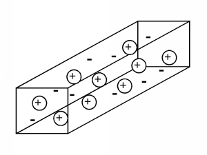
As shown in Figure \(\PageIndex{1}\), the model of the conductor consists of a number of mobile positive charges (represented by the balls with the "+" sign in them) and an equal number of fixed negative charges (represented by the bare "-" sign). In subsequent figures, we will leave out the fixed charge, since it can not contribute in any way to the conduction process, but keep in mind that it is there, and that the total net charge is zero within the material. Each of the mobile charge carriers has a mass, \(m\), and an amount of charge, \(q\).
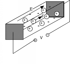
In order to have some conduction, we have to apply a potential or voltage across the sample (Figure \(\PageIndex{2}\)). We do this with a battery, which creates a potential difference, \(V\), between one end of the sample and the other. We will make the simplest assumption that we can, and say that the voltage, \(V\), gives rise to a uniform electric field within the sample. The magnitude of the electric field is given simply by \[E = \frac{V}{L} \nonumber \] where \(L\) is the length of the sample, and \(V\) is the voltage which is placed across it. (In truth, we should be showing \(E\) as well as subsequent forces, etc. as vectors in our equations, but since their direction will be obvious and unambiguous, let's keep things simple, and just write them as scalars.) Electric potential, or voltage, is just a measure of the change in potential energy per unit charge going from one place to another. Since energy, or work is simply force times distance, if we divide the energy per unit charge by the distance over which that potential exists, we will end up with force per unit charge, or electric field, \(E\). If you are not sure about what you just read, write it out as equations, and see that it is so.
The electric field will exert a force on the movable charges (and the fixed ones too, for that matter, but since they can not go anywhere, nothing happens to them). The force is given simply as the product of the electric field strength times the charge: \[F = qE \nonumber \]
The force acts on the charges and causes them to accelerate according to Newton's equations of motion: \[\begin{array}{l} F &= \ m \dfrac{dv}{dt} \\ &= \ qE \end{array} \nonumber \] or \[\frac{d}{dt} v(t) = \frac{qE}{m} \nonumber \]
Thus, the velocity of a particle with no initial velocity will increase linearly with time as: \[v(t) = \frac{qE}{m} t \nonumber \] The rate of acceleration is proportional to the strength of the electric field, and inversely proportional to the mass of the particle. However, the particle can not continue to accelerate forever. Since it is located within a solid, sooner or later it will collide with either another carrier, or perhaps one of the fixed atoms within the solid. We will assume that the collision is completely inelastic, and that after a collision, the particle comes to a stop, only to be accelerated again by the electric field. If we were to make a plot of the particle's velocity as a function of time, it might look something like Figure \(\PageIndex{3}\).
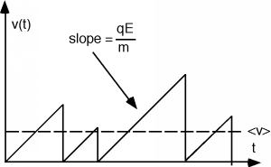
Although the particle achieves various velocities, depending upon how much time there is between collisions, there will be some average velocity, \(\bar{v}\), which will depend upon the details of the collision process. Let us define a scattering time \(\tau_{s}\) which will give us that average velocity when we multiply it by the acceleration of the particle. That is, \[\bar{v} = \frac{q E \tau_{s}}{m} \nonumber \] or \[\tau_{s} = \frac{m \bar{v}}{qE} \nonumber \]
Now let's take a look at just a small section of the conductor (Figure \(\PageIndex{4}\)). It will have the cross section of the sample, \(A\), but will only be \(\bar{v} \Delta t\) long, where \(\Delta (t)\) is just some arbitrary time interval.
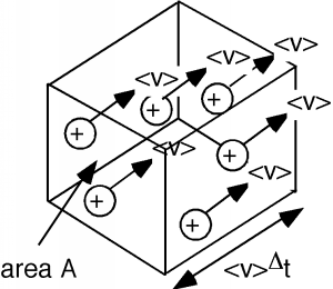
After a time \(\Delta (t)\) has passed, all of the charges within the box will have left it, as they are all moving with the same average velocity \(\bar{v}\). If the density of charge carriers in the conductor is \(n\) per unit volume, then the number of carriers \(N\) within our little box is just \(n\) times the volume of the box, \(\bar{v} \Delta (t) A\). \[N = n \bar{v} \Delta (t) A \nonumber \]
Thus the total charge \(Q\) which leaves the box in time \(\Delta (t)\) is just \(qN\). The current flow, \(I\), is just the amount of charge which flows out of the box per unit time: \[\begin{array}{l} I &= \ \dfrac{q n v \Delta(t) A}{\Delta (t)} \\ &= \ qn \bar{v} A \\ &= \ \dfrac{q_{2} n \tau_{s} EA}{m} \\ &= \ \dfrac{Q}{\Delta (t)} \end{array} \nonumber \]
We now have two choices. We can look at our result from a field quantity point of view, in which case we will be interested in the current density, \(J\), which is just the current, \(I\), divided by the cross-sectional area: \[\begin{array}{l} J &= \ \dfrac{I}{A} \\ &= \ \dfrac{q^{2} n \tau_{s}}{m} E \\ &= \ \sigma E \end{array} \nonumber \]
where \(\sigma\) is called the conductivity of the material. If we look at the conductor from a macroscopic point of view, then we are interested in the relationship between the voltage and the current. The voltage is just the electric field times the length of the sample, and the current is just the current density times its cross-sectional area. Thus we have \[\begin{array}{l} I &= \ AJ \\ &= \ A \sigma E \\ &= \ A \sigma \dfrac{V}{L} \end{array} \nonumber \] or \[\begin{array}{l} V &= \ \dfrac{L}{\sigma A} I \\ &= \ RI \end{array} \nonumber \]
where \(R\) is the resistance of the sample. We have discovered Ohm's law!
Note that Equation \(\PageIndex{13}\) tells us that the resistance of the sample is proportional to its length (the longer the sample, the higher the resistance) and inversely proportional to its cross-sectional area (the fatter the sample, the lower the resistance). The sample resistance is also inversely proportional to the conductivity \(\sigma\) of the sample. Sometimes, instead of conductivity, the resistivity, \(\rho\), is specified for a resistive material. The resistivity is simply the inverse of the conductivity: \[\sigma = \frac{1}{\rho} \nonumber \] Thus, \[R = \frac{\rho L}{A} \nonumber \]
And, in an effort towards completeness, there is one other quantity which you might run into, and that is the carrier mobility, \(\mu\). The mobility is just the proportionality factor between the average velocity of the particle and the electric field. That is: \[\bar{v} = \mu E \nonumber \]
You should check that the following two relationships are correct: \[\begin{align} \sigma &= n q \mu \\ { } \nonumber \\ \mu &= \frac{q \tau_{s}}{m} \end{align} \nonumber \] If we take an ordinary conductor (we will have to define later what we mean by that) and heat it up, the atoms within the material start to vibrate faster due to the elevated temperature, and the carriers suffer significantly more collisions. The mean collision time \(\tau_{s}\) decreases, and hence the conductivity goes down, and the resistance of the sample goes up.