3.4.6: Plotting MOS I-V

Last updated
Save as PDF

Page ID: 89973

\( \newcommand{\vecs}[1]{\overset { \scriptstyle \rightharpoonup} {\mathbf{#1}} } \) \( \newcommand{\vecd}[1]{\overset{-\!-\!\rightharpoonup}{\vphantom{a}\smash {#1}}} \)\(\newcommand{\id}{\mathrm{id}}\) \( \newcommand{\Span}{\mathrm{span}}\) \( \newcommand{\kernel}{\mathrm{null}\,}\) \( \newcommand{\range}{\mathrm{range}\,}\) \( \newcommand{\RealPart}{\mathrm{Re}}\) \( \newcommand{\ImaginaryPart}{\mathrm{Im}}\) \( \newcommand{\Argument}{\mathrm{Arg}}\) \( \newcommand{\norm}[1]{\| #1 \|}\) \( \newcommand{\inner}[2]{\langle #1, #2 \rangle}\) \( \newcommand{\Span}{\mathrm{span}}\) \(\newcommand{\id}{\mathrm{id}}\) \( \newcommand{\Span}{\mathrm{span}}\) \( \newcommand{\kernel}{\mathrm{null}\,}\) \( \newcommand{\range}{\mathrm{range}\,}\) \( \newcommand{\RealPart}{\mathrm{Re}}\) \( \newcommand{\ImaginaryPart}{\mathrm{Im}}\) \( \newcommand{\Argument}{\mathrm{Arg}}\) \( \newcommand{\norm}[1]{\| #1 \|}\) \( \newcommand{\inner}[2]{\langle #1, #2 \rangle}\) \( \newcommand{\Span}{\mathrm{span}}\)\(\newcommand{\AA}{\unicode[.8,0]{x212B}}\)

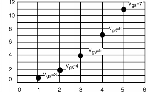
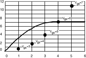
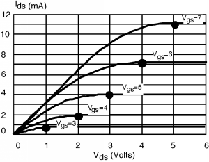
Once we have the numbers (Table \(\PageIndex{1}\), then we sketch a piece of graph paper with the proper scale, and plot the points on it. Once the \(\left(I_{\text{d sat}}, \ V_{\text{d sat}}\right)\) points have been determined, it is easy to sketch in the \(I\text{-}V\) behavior. You just draw a curve from the origin up to any given point, having it "peak out" just at the dot, and then draw a straight line at \(I_{\text{d sat}}\) to finish things off. One such curve is shown in Figure \(\PageIndex{2}\). And then finally in Figure \(\PageIndex{3}\) they are all sketched in. Your curves probably won't be exactly right but they will be good enough for a lot of applications.

Table \(\PageIndex{1}\): Results of calculating \(V_{\text{d sat}}\) and \(I_{\text{d sat}}\)
\(V_{\text{gs}}\)	\(V_{\text{d sat}} \ (\mathrm{V})\)	\(I_{\text{d sat}} \ (\mathrm{mA})\)
\(3\)	\(1\)	\(0.44\)
\(4\)	\(2\)	\(1.76\)
\(5\)	\(3\)	\(3.96\)
\(6\)	\(4\)	\(7.04\)
\(7\)	\(5\)	\(11\)

Points from Table 3.6.1, plotted on an x-axis of V_dsat in volts and a y-axis of I_dsat in milliamps. — Figure \(\PageIndex{1}\): Plotting \(I_{\text{d sat}}\) and \(V_{\text{d sat}}\).

One of the I-V curves is drawn into the plot from Figure 1 above. A concave-down curve starts at the origin and reaches its maximum at the V_gs=6 point, and smoothly transitions to a straight horizontal line to the right. — Figure \(\PageIndex{2}\): Sketching in one of the \(I\text{-}V\) curves.

I-V curves drawn in for all the plotted points from the table above. Each curve follows the pattern of its plotted point forming the maximum of a concave-down curve starting from the origin, smoothly transitioning into a horizontal line for larger values of V_dsat. — Figure \(\PageIndex{3}\): The complete set of curves.

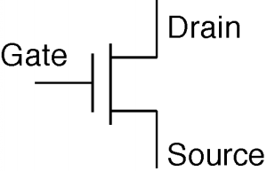
There is a particularly easy way to measure by \(k\) and \(V_{t}\) for a MOSFET. Let's first introduce the schematic symbol for the MOSFET; it looks like Figure \(\PageIndex{4}\). Let's take a MOSFET and hook it up as shown in Figure \(\PageIndex{5}\).

A MOSFET schematic symbol for a circuit diagram. The gate is represented by a short horizontal line, its right endpoint intersecting the midpoint of a short vertical line. A short distance to the right is a longer vertical line. Two short horizontal lines extend from this line, to the right. A vertical line extends upwards from the right end of the upper horizontal line; this represents the drain. Another vertical line extends down from the right end of the lower horizontal line; this represents the source. — Figure \(\PageIndex{4}\): Schematic symbol for a MOSFET

A voltage source has current I_d flowing out of its positive end and entering a junction where one branch connects to the gate of a MOSFET and the other branch connects to the MOSFET's drain. The MOSFET's source is connected to the negative end of the voltage source. There is a voltage drop of V_ds between the drain and the source. — Figure \(\PageIndex{5}\): Circuit for finding \(V_{t}\) and \(k\)

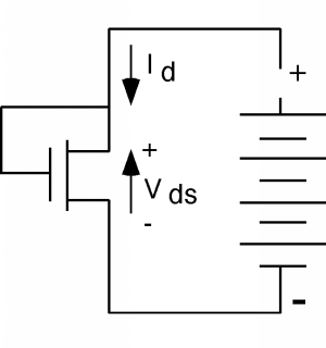
Since the gate of this transistor is connected to the drain, there is no doubt that \(V_{\text{gs}} - V_{\text{ds}}\) is less than \(V_{t}\). In fact, since \(V_{\text{gs}} = V_{\text{ds}}\), their difference is zero. Thus, for any value of \(V_{\text{ds}}\), this transistor is operating in its saturated condition. Since \(V_{\text{gs}} = V_{\text{ds}}\), we can rewrite a previous equation derived equation from the section on MOS regimes as \[I_{d} = \frac{k}{2} \left(V_{\text{ds}} - V_{t}\right)^{2}\]

Now let's take the square root of both sides: \[\sqrt{I_{d}} = \sqrt{\frac{k}{2}} \left(V_{\text{ds}} - V_{t}\right)\]

So if we make a plot of \(\sqrt{I_{d}}\) as a function of \(V_{\text{ds}}\), we should get a straight line, with a slope of \(\sqrt{\frac{k}{2}}\) and an \(x\)-intercept of \(V_{t}\).

The graph of the square root of I_d vs V_ds, in the first quadrant, takes the form of a small concave-up curve rising from a point along the x-axis smoothly transitioning into a line whose slope is the square root of one-half of k. If this linear portion of the graph is extended, it intercepts the x-axis at the point V_T. — Figure \(\PageIndex{6}\): Obtaining \(V_{t}\) and \(k\)

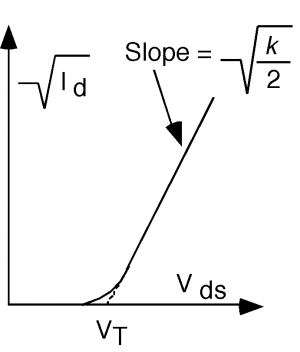
Because of the expected non-ideality, the curve does not go all the way to \(V_{t}\), but deviates a bit near the bottom. A simple linear extrapolation of the straight part of the plot however, yields an unambiguous value for the threshold voltage \(V_{t}\).