9.5.5: Fick's Second Law
- Page ID
- 89985

Taking the derivative with respect to \(x\) of Fick's first law \[\frac{\text{d}}{\text{d} x} (\text{Flux}) = - \left( D \frac{\partial^{2} N(x, t)}{\partial x_{2}^{ 2}} \right)\]
and then substituting the continuity equation into it, we have Fick's second law of diffusion: \[\frac{\partial N(x, t)}{\partial t} = D \frac{\partial^{2} N(x, t)}{\partial x_{2}^{ 2}}\]
This is a standard diffusion equation, and one which shows up over and over again when one is dealing with such phenomena.
In order to get a solution to the diffusion equation, we must first assume some boundary conditions. We will deal with a semi-infinite wafer, and assume that \[\lim_{x \rightarrow \infty} N(x, t) = 0\]
This is a reasonable assumption, since at most our diffusion will only penetrate a micron or so into the wafer, and the whole wafer itself is several hundred microns thick.
We also have to decide something about initial conditions. We will make the assumption that we have at time \(t=0\) and \(x=0\) some surface concentration of impurities which we will call \(Q_(0)\), measured in \(\frac{\mathrm{impurities}}{\mathrm{cm}^2}\). This is the situation we would have if we introduce the impurities using a relatively shallow implant step. An alternative surface boundary condition would be one where the concentration of impurities remains at some fixed value. This is what happens when there are impurities in the gas flow over the wafer during the time that they are in the diffusion oven. This is called an infinite source diffusion.
The first condition is called a limited source diffusion, and that is what we shall consider further here. It is not too hard to show that with this initial condition, the solution to the diffusion equation is: \[N(x, t) = \frac{Q_{0}}{\sqrt{\pi Dt}} e^{- \frac{x^{2}}{4Dt}}\]
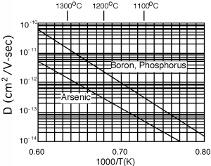
Note that \(N(x, t)\) is a function of distance into the wafer \(x\) and time \(t\). The time is, of course, the time of the diffusion process. \(D\), the diffusion constant, depends on the temperature at which the diffusion takes place. Figure \(\PageIndex{1}\) is a plot of \(D\) for three of the most commonly used dopants in silicon. Phosphorus and boron are the most common acceptor and donor respectively. Arsenic is sometimes used because it is significantly bigger in diameter than either phosphorus or boron, and thus moves around less after an implant.
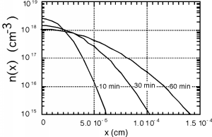
Suppose we do a relatively shallow implant of boron into our p-type wafer, and deposit a \(Q_{0}\) of \(5 \times 10^{13}\) phosphorus \(\frac{\mathrm{atoms}}{\mathrm{cm}^2}\). We then perform an anneal diffusion at \(1100 ^{\circ} \mathrm{C}\) for 60 minutes. At \(1100 ^{\circ} \mathrm{C}\), \(D\) for phosphorus seems to be about \(2 \times 10^{-13} \ \frac{\mathrm{cm}^2}{\mathrm{sec}}\). We will make a plot of \(N(x)\) for various times. If you do this at home, be sure to put time in seconds, not minutes, hours, or fortnights. Looking at Figure \(\PageIndex{2}\), it is pretty easy to see how the impurities move into the semiconductor, and how the concentration at the surface, \(N(0, t)\), decreases as more and more of the impurities move deeper into the wafer.