4.5.2: Forces on Curved Surfaces

Fig. 4.26. The forces on curved area.

The pressure is acting on surfaces perpendicular to the direction of the surface (no shear forces assumption). The element force is \[d\bf{F} = -P\hat{n}\bf{dA} \] Here, the conventional notation is used which is to denote the area, \(dA\), outward as positive. The total force on the area will be the integral of the unit force \[\bf{F} = -\int_{A}P\hat{n}\bf{dA} \] The result of the integral is a vector. So, if the \(y\) component of the force is needed, only a dot product is needed as \[dF_{y} = d\bf{F}\bf{\cdot}\hat{j}\] From this analysis (eqn. 180) it can be observed that the force in the direction of \(y\), for example, is simply the integral of the area perpendicular to \(y\) as \[F_{y} = \int_{A} P dA_{y}\] The same can be said for the \(x\) direction. The force in the \(z\) direction is \[F_{z} = \int_{A} h g \rho d A_{z} \]

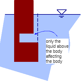
Fig. 4.27. Schematic of net force on floating body.

The force which acting on the \(z\) direction is the weight of the liquid above the projected area plus the atmospheric pressure. This force component can be combined with the other components in the other directions to be \[F_{total} = \sqrt{F_{z}^{2} + F_{x}^{2} + F_{y}^{2}} \] The angle in \(xz\) plane is \[tan\theta_{xz} = \frac{F_{z}}{F_{x}}\] and the angle in the other plane, \(yz\) is \[tan \theta_{zy} = \frac{F_{z}}{F_{y}}\]

The moment due to the curved surface require integration to obtain the value. There are no readily made expressions for these 3–dimensional geometries. However, for some geometries there are readily calculated center of mass and when combined with two other components provide the moment (force with direction line).

Cut–Out Shapes Effects

There are bodies with a shape that the vertical direction ( \(z\) direction) is "cut-out" aren't continuous. Equation 182 implicitly means that the net force on the body is \(z\) direction is only the actual liquid above it. For example, Figure 4.27 shows a floating body with cut–out slot into it. The atmospheric pressure acts on the area with continuous lines. Inside the slot, the atmospheric pressure with it piezometric pressure is canceled by the upper part of the slot. Thus, only the net force is the actual liquid in the slot which is acting on the body. Additional point that is worth mentioning is that the depth where the cut–out occur is insignificant (neglecting the change in the density).

Example 4.17

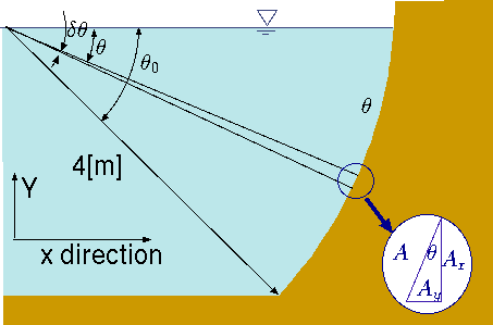
Fig. 4.28 Calculations of forces on a circular shape dam.

Calculate the force and the moment around point "O'' that is acting on the dam (see Figure (4.28)). The dam is made of an arc with the angle of \(\theta_0=45^∘\) and radius of \(r=2[m]\). You can assume that the liquid density is constant and equal to \(1000 [kg/m^3]\). The gravity is 9.8\([m/sec^2]\) and width of the dam is \(b=4[m]\). Compare the different methods of computations, direct and indirect.

Solution 4.17

The force in the \(x\) direction is
\begin{align*}
F_x = \int_{A} P \overbrace{r\,\cos\theta\,d\theta}^{dA_x}
\end{align*}
Note that the direction of the area is taken into account (sign). The differential area that will be used is, \(b\,r\,d\theta\) where \(b\) is the width of the dam (into the page). The pressure is only a function of \(\theta\) and it is
\begin{align*}
P = P_{atmos} + \rho \, g \, r \sin\theta
\end{align*}
The force that is acting on the \(x\) direction of the dam is \(A_x \times P\). When the area \(A_x\) is \(b\,r\,d\theta \,\cos\theta\). The atmospheric pressure does cancel itself (at least if the atmospheric pressure on both sides of the dam is the same). The net force will be
\begin{align*}
F_x = \int_0^{\theta_0} \overbrace{\rho \,g\,r\,\sin\theta}^{P}
\overbrace{\,b\,r\,\cos \theta\,d\theta}^{dA_x}
\end{align*}
The integration results in

Area Arc Subtract the Triangle
Fig. 4.29 Area above the dam arc subtract triangle.

\begin{align*}
F_x = \dfrac{\rho\,g\,b\,r^2}{2}\,
\left(1-{cos^{2}\left( \theta_ 0\right) } \right)
\end{align*}
Alternative way to do this calculation is by calculating the pressure at mid point and then multiply it by the projected area, \(A_x\) (see Figure 4.29) as
\begin{align*}
F_x = \rho\,g\,\overbrace{b\,r\sin\theta_0}^{A_x}
\overbrace{\dfrac{r\sin\theta_0}{2}}^{x_c}
= \dfrac{\rho\,g\,b\,r}{2}\, \sin^2\theta
\end{align*}
Notice that \(dA_x\)(\(\cos\theta\)) and \(A_x\) (\(\sin\theta\)) are different, why? The values to evaluate the last equation are provided in the question and simplify subsidize into it as
\begin{align*}
F_x = \dfrac{1000\times 9.8\times 4 \times 2}{2} \sin(45^{\circ})
= 19600.0 [N]
\end{align*}
Since the last two equations are identical (use the sinuous theorem to prove it \( \sin^2\theta + \cos^2 = 1\)), clearly the discussion earlier was right (not a good proof The force in the \(y\) direction is the area times width.
\begin{align*}
F_y = - \overbrace{\left(\overbrace{\dfrac{\theta_0\,r^2}{2}-
\dfrac{r^2\sin\theta_0\cos\theta_0}{2}}^{A}\right) \,b}^{V}
\,g\, \rho
\sim 22375.216[N]
\end{align*}
The center area (purple area in Figure 4.29) should be calculated as
\begin{align*}
y_c = \dfrac

ParseError: EOF expected (click for details)

Callstack:
    at (Bookshelves/Civil_Engineering/Book:_Fluid_Mechanics_(Bar-Meir)/04:_Fluids_Statics/4.5:_Fluid_Forces_on_Surfaces/4.5.2:_Forces_on_Curved_Surfaces), /content/body/div[1]/div[2]/p[4]/span, line 1, column 4

{A}
\end{align*}
The center area above the dam requires to know the center area of the arc and triangle shapes. Some mathematics are required because the shift in the arc orientation. The arc center (see Figure 4.30) is at
\begin{align*}
{y_c}_{arc} = \dfrac{4\,r \sin^2\left(\dfrac{\theta}{2} \right)} {3\,\theta}
\end{align*}

Arc Center in the y direction
Fig. 4.30 Area above the dam arc calculation for the center.

All the other geometrical values are obtained from Tables and (??). and substituting the proper values results in
\begin{align*}
{y_c}_r = \dfrac{\overbrace{\dfrac{\theta\,r^2}{2}}^{A_{arc}}
\overbrace{ \dfrac{4\,r \sin\left(\dfrac{\theta}{2} \right)
\cos\left(\dfrac{\theta}{2}\right) }
{3\,\theta} }^{y_c} -
\overbrace{\dfrac{2\,r\,\cos\theta}{3}}^{y_c}
\overbrace{\dfrac{\sin\theta\,r^2}{2}}^{A_{triangle}} }
{\underbrace{\dfrac{\theta\,r^2}{2}}_{A_{arc}} -
\underbrace {\dfrac{r^2\,\sin\theta\,\cos\theta}{2}}_{A_{triangle}}}
\end{align*}
This value is the reverse value and it is
\begin{align*}
{y_c}_r = 1.65174[m]
\end{align*}
The result of the arc center from point "O'' (above
calculation area) is
\begin{align*}
y_c = r - {y_c}_{r} = 2 - 1.65174 \sim 0.348[m]
\end{align*}
The moment is
\begin{align*}
M_v = y_c \,F_y \sim 0.348\times 22375.2
\sim 7792.31759
[N\times m]
\end{align*}
The center pressure for \(x\) area is
\begin{align*}
x_p = x_c + \dfrac{I_{xx} }{x_c\,A} =
\dfrac{r\,cos\theta_0}{2} +
\dfrac{\overbrace{\dfrac{\cancel{b}\,\left(r\cos\theta_0\right)^3}
{36}}^{I_{xx}}}
{\underbrace{\dfrac{r\,cos\theta_0}{2}}_{x_c}
\cancel{b}\left(r\,\cos\theta_0\right)} =
\dfrac{5\,r\cos\theta_0}{9}
\end{align*}
The moment due to hydrostatic pressure is
\begin{align*}
M_h = x_p \, F_x = \dfrac{5\,r\,cos\theta_0}{9} \,F_x
\sim 15399.21[N\times m]
\end{align*}
The total moment is the combination of the two and it is
\begin{align*}
M_{total} = 23191.5 [N\times m]
\end{align*}

Moment on Arc Element
Fig. 4.31 Moment on arc element around Point "O.''

For direct integration of the moment it is done as following
\begin{align*}
dF = P\,dA = \int_0^{\theta_0} \rho \, g\, \sin\theta
\,b\,r\,d\theta
\end{align*}
and element moment is
\begin{align*}
dM = dF \times ll = dF
\overbrace{2\,r\,\sin\left(\dfrac{\theta}{2} \right)}^{ll}
\cos\left(\dfrac{\theta}{2} \right)
\end{align*}
and the total moment is
\begin{align*}
M = \int_0^{\theta_0} dM
\end{align*}
or
\begin{align*}
M =
\int_0^{\theta_0}
\rho \, g\, \sin\theta \,b\,r\,
{2\,r\,\sin\left(\dfrac{\theta}{2} \right)}
\cos\left(\dfrac{\theta}{2} \right) d\theta
\end{align*}
The solution of the last equation is
\begin{align*}
M = \dfrac{g\,r\,\rho\,
\left( 2\,\theta_0 - \sin\left( 2\,\theta_0\right) \right) }{4}
\end{align*}
The vertical force can be obtained by
\begin{align*}
F_v = \int_0^{\theta_0}P\,dA_v
\end{align*}
or
\begin{align*}
F_v = \int_0^{\theta_0} \overbrace{\rho\,g\, r\,\sin\theta}^{P}
\overbrace{r\,d\theta\,\cos\theta}^{dA_v}
\end{align*}
\begin{align*}
F_v = \dfrac{g\,{r}^{2}\,\rho}{2}
\,\left( 1 -

ParseError: EOF expected (click for details)

Callstack:
    at (Bookshelves/Civil_Engineering/Book:_Fluid_Mechanics_(Bar-Meir)/04:_Fluids_Statics/4.5:_Fluid_Forces_on_Surfaces/4.5.2:_Forces_on_Curved_Surfaces), /content/body/div[1]/div[2]/p[8]/span, line 1, column 4

\right)
\end{align*}
Here, the traditional approach was presented first, and the direct approach second. It is much simpler now to use the second method. In fact, there are many programs or hand held devices that can carry numerical integration by inserting the function and the boundaries.

To demonstrate this point further, consider a more general case of a polynomial function. The reason that a polynomial function was chosen is that almost all the continuous functions can be represented by a Taylor series, and thus, this example provides for practical purposes of the general solution for curved surfaces.

Example 4.18

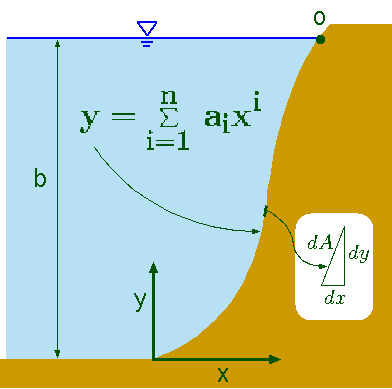
Fig. 4.32 Polynomial shape dam description for the moment around point ``O'' and force calculations.

For the liquid shown in Figure ,calculate the moment around point "O'' and the force created by the liquid per unit depth. The function of the dam shape is \(y = \sum_{i=1}^n a_i\,x^i\) and it is a monotonous function (this restriction can be relaxed somewhat). Also calculate the horizontal and vertical forces.

Solution 4.18

The calculations are done per unit depth (into the page) and do not require the actual depth of the dam. The element force (see Figure 4.32) in this case is

\[ dF = \overbrace{\overbrace{(b-y)}^{h}\,g\,\rho}^{P}
\overbrace{\sqrt{dx^2 + dy^2}}^{dA}
\]

The size of the differential area is the square root of the \(dx^2\) and \(dy^2\) (see Figure 4.3). It can be noticed that the differential area that is used here should be multiplied by the depth. From mathematics, it can be shown that

\[ \sqrt{dx^2 + dy^2} = dx\,\sqrt{1+ \left(\dfrac{dy}{dx}\right)^2}
\]

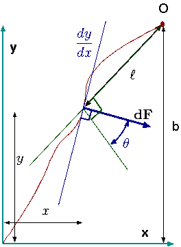
Fig. 4.33 The difference between the slop and the direction angle.

The right side can be evaluated for any given function. For example, in this case describing the dam function is
\begin{align*}
\sqrt{1+ \left(\dfrac{dy}{dx}\right)^2} =
\sqrt{ 1 +
{\left( \sum_{i=1}^{n}i\,a\left( i\right) \,{x\left( i\right) }
^{i-1}\, \right) }^{2} }
\end{align*}
The value of \(x_b\) is where \(y=b\) and can be obtained by finding the first and positive root of the equation of
\begin{align*}
0 = \sum_{i=1}^n a_i\,x^i - b
\end{align*}
To evaluate the moment, expression of the distance and angle to point "O'' are needed (see Figure 4.33). The distance between the point on the dam at \(x\) to the point "O'' is
\begin{align*}
ll(x) = \sqrt{(b-y)^2+ (x_b-x)^2 }
\end{align*}
The angle between the force and the distance to point "O'' is
\begin{align*}
\theta(x) = \tan^{-1}\left(\dfrac{dy}{dx}\right) -
\tan^{-1}\left(\dfrac{b-y}{x_b-x}\right)
\end{align*}
The element moment in this case is
\begin{align*}
dM = ll(x)\,
\overbrace{(b-y)\,g\,\rho\,\sqrt{1+
\left(\dfrac{dy}{dx}\right)^2}}^{dF}
\,\cos\theta(x)\, dx
\end{align*}
To make this example less abstract, consider the specific case of \(y = 2\,x^6\). In this case, only one term is provided and \(x_b\) can be calculated as following
\begin{align*}
x_b = \sqrt[6]{\dfrac{b}{2}}
\end{align*}
Notice that \( \sqrt[6]{\dfrac{b}{2}}|) is measured in meters. The number "2'' is a dimensional number with units of [1/\(m^5\)]. The derivative at \(x\) is
\begin{align*}
\dfrac{dy}{dx} = 12\,x^5
\end{align*}
and the derivative is dimensionless (a dimensionless number).
The distance is
\begin{align*}
ll = \sqrt{\left(b -2\,x^6\right)^2 +
\left( \sqrt[6]{\dfrac{b}{2}} - x \right)^2}
\end{align*}
The angle can be expressed as
\begin{align*}
\theta = \tan^{-1}\left(12\,x^5\right) -
\tan^{-1}\left(\dfrac{b- 2\,x^6}{\sqrt[6]{\dfrac{b}{2}} -x}\right)
\end{align*}
The total moment is
\begin{align*}
M = \int_0^{\sqrt[6]{b}} ll(x) \cos\theta(x)
\left( b-2\,x^6 \right)\,g\,\rho
\sqrt{1+12\,x^5}\;dx
\end{align*}
This integral doesn't have a analytical solution. However, for a given value \(b\) this integral can be evaluate. The horizontal force is
\begin{align*}
F_h = b\,\rho\,g \,\dfrac{b}{2} = \dfrac{\rho\,g\,b^2}{2}
\end{align*}
The vertical force per unit depth is the volume above the dam as
\begin{align*}
F_v = \int_0^{\sqrt[6]{b}} \left(b - 2\,x^6\right) \rho
\,g\,dx = \rho \,g\,\dfrac{5\,{b}^{\dfrac{7}{6}}}{7}
\end{align*}
In going over these calculations, the calculations of the center of the area were not carried out. This omission saves considerable time. In fact, trying to find the center of the area will double the work. This author find this method to be simpler for complicated geometries while the indirect method has advantage for very simple geometries.

Contributors and Attributions

• Dr. Genick Bar-Meir. Permission is granted to copy, distribute and/or modify this document under the terms of the GNU Free Documentation License, Version 1.2 or later or Potto license.