10.3.1: Flow Around a Circular Cylinder

After several elements of the potential flow were built earlier, the first use of these elements can be demonstrated. Perhaps the most celebrated and useful example is the flow past a cylinder which this section will be dealing with. The stream function made by superimposing a uniform flow and a doublet is

\[ \label{if:eq:stream-U+doublet1}
\psi = U_0 \, y + \dfrac {Q_0}{2\,\pi} \dfrac{\sin\theta}{r} =
U_0 \, r\, \sin\theta + \dfrac {Q_0}{2\,\pi} \dfrac{r\,\sin\theta}{r^2}
\]

Or after some arrangement equation (91) becomes

\[ \label{if:eq:stream-U+doublet2}
\psi = U_0 \, r\, \sin\theta \left(1 + \dfrac {Q_0}{2\,U_0\,\pi\,r^2} \right)
\] Denoting \(\dfrac {Q_0}{2\,U_0\,\pi}\) as \(-a^2\) transforms equation (92) to

\[ \label{if:eq:stream-U+doublet3}
\psi = U_0 \, r\, \sin\theta \left(1 - \dfrac {a^2}{r^2} \right)
\] The stream function for \(\psi=0\) is

\[ \label{if:eq:stream0-U+doublet}
0 = U_0 \, r\, \sin\theta \left(1 - \dfrac {a^2}{r^2} \right)
\] This value is obtained when \(\theta=0\) or \(\theta = \pi\) and/or \(r=a\). The stream line that is defined by radius \(r=a\) describes a circle with a radius \(a\) with a center in the origin. The other two lines are the horizontal coordinates. The flow does not cross any stream line, hence the stream line represented by \(r=a\) can represent a cylindrical solid body. For the case where \(\psi e 0\) the stream function can be any value. Multiplying equation (93) by \(r\) and dividing by \(U_0\,a^2\) and some rearranging yields

\[ \label{if:eq:stream-U+doublet3intermidiatIni}
\dfrac{r}{a}\,\dfrac{\psi}{a\,U_0} = \left(\dfrac{r}{a}\right)^2\, \sin\theta - \sin\theta
\] It is convenient, to go through the regular dimensionalzing process as

\[ \label{if:eq:stream-U+doublet3intermidiat}
\overline{r}\,\overline{\psi} = (\overline{r})^2\, \sin\theta - \sin\theta \quad
\text{or}\quad \overline{r}^2 - \dfrac{\overline{\psi}}{\sin\theta} \, \overline{r}-1 = 0
\] The radius for other streamlines can found or calculated for a given angle and given value of the stream function. The radius is given by

\[ \label{if:stream0-U+doubletR}
\overline{r} = \dfrac{\dfrac{\overline{\psi}}{\sin\theta}\pm
\sqrt{ \left( \dfrac{\overline{\psi}}{\sin\theta} \right)^2+4} }
{2}
\] It can be observed that the plus sign must be used for radius with positive values (there are no physical radii which negative absolute value). The various value of the stream function can be chosen and drawn. For example, choosing the value of the stream function as multiply of \(\overline{\psi} = 2\,n\) (where \(n\) can be any real number) results in

\[ \label{if:eq:streamaU0-U+doubletRIni}
\overline{r} = \dfrac{\dfrac{2\,n}{\sin\theta}\pm
\sqrt{ \left( \dfrac{2\,n}{\sin\theta} \right)^2+4} }
{2} =
n\, \text{csc}(\theta) + \sqrt{n^2\,\text{csc}^2(\theta) + 1}
\] The various values for of the stream function are represented by the ratios \(n\). For example for \(n=1\) the (actual) radius as a function the angle can be written as

\[ \label{if:eq:streamaU0-U+doubletR}
r = a\,\left( \text{csc}(\theta) + \sqrt{\text{csc}^2(\theta) + 1} \right)
\] The value csc\((\theta)\) for \(\theta= 0 \,\, \text{and} \,\, \theta = \pi\) is equal to infinity (\(\infty\)) and for values of csc\((\theta=\pi/2) = 1\). Similar every line can be evaluated. The lines are drawn in Figure 10.13.

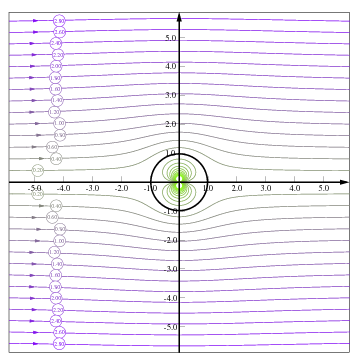
Fig. 10.13 Stream function of uniform flow plus doublet results in solid body with flow around it. Stream function (\(n\) and not \(\psi\)) starts from -2.0 (green line) to 3 the (purple line). The negative streamlines lines are inside the solid body. The arrows are calculated by trapping the \(y\) for given \(\psi\) around the end points. Hence, the slight difference between the arrow and the line. The more negative the stream function the smaller the counter. The larger positive stream function the further away the line form the \(x\) coordinate. It can be noticed closer the solid body'' the lines are more curved. The GLE code is attached in the source code to this book. The value of \(n\) is the bubbles.

The velocity of this flow field can be found by using the equations that were developed so far. The radial velocity is

\[ \label{if:eq:unifomDoubletUr}
U_r = \dfrac{1}{r} \dfrac{\partial \psi}{\partial \theta} =
U_0 \,\cos \theta \, \left( 1 - \dfrac{a^2}{r^2}\right)
\]

The tangential velocity is

\[ \label{if:eq:unifomDoubletUtheta}
U_r = - \dfrac{\partial \psi}{\partial r} =
U_0 \,\sin \theta \, \left( 1 + \dfrac{a^2}{r^2}\right)
\]

Example 10.7

A sink is placed in a uniform flow field from the left to right. Describe flow field by the stream lines. Find the shape of the solid body described by this flow.

Solution 10.7

The stream function for uniform flow is given by equation (7) and the stream by equation (17) (with positive sign because it is source). Hence the stream function is

\[ \label{uniformSource:streamF}
\psi = U_0\,r\,\sin\theta + \dfrac{\dot{Q}} {2\,\pi}\,\theta
\]

For \(\psi=0\) equation (102) becomes

\[ \label{uniformSource:psi0}
r = - \dfrac{\dot{Q}\,\theta} {2\,\pi\,U_0\,\sin\theta}
\] or in for any value of stream function, \(\psi\) as

\[ \label{uniformSource:psi}
r = \dfrac{\psi}{U_0\,\sin\theta} - \dfrac{\dot{Q}\,\theta} {2\,\pi\,U_0\,\sin\theta}
\] The long cigar shape resulted from the combination of the uniform flow with the source is presented in Figure 10.14. The black line represents the solid body that created and show two different kind of flows. The exterior and the interior flow represent the external flow outside and the inside the black line represents the flow on the enclosed body. The black line divides the streamline, which separates the fluid coming from the uniform source the flow due to the inside source. Thus, these flows represent a flow around semi–infinite solid body and flow from a source in enclosed body.

Fig. 10.14 Source in the Uniform Flow.

The width of the body at infinity for incompressible flow can be determined by the condition that the flow rate must be the same. The velocity can be obtained from the stream function. Substituting into (103) as

\[ \label{uniformSource:psi0y}
\overbrace{y}^{r\,\sin\theta} = - \dfrac{\dot{Q}\,\theta} {2\,\pi\,U_0}
\]

An noticing that at \(\theta=\pi\) is on the right hand side (opposite to your the intuition) of the solid body (or infinity). Hence equation (105) can be written as

\[ \label{uniformSource:yatInifinity}
y = \dfrac{\dot{Q}\,\cancel{\pi}} {2\,\cancel{\pi}\,U_0}
= \dfrac{\dot{Q}} {2\,U_0}
\] It can be noticed that sign in front of \(y\) is accounted for and thus removed from the equation. To check if this analysis is consistent with the continuity equation, the velocity at infinity must be \(U=U_0\) because the velocity due to the source is reduced as \(\sim 1/r\). Hence, the source flow rate must must be balanced (see for the integral mass conservation) flow rate at infinity hence

\[ \label{uniformSource:eq:infinityFlowRate}
Q = U_0 \,2\,y = U_0 \,2\, \dfrac{Q_0} {2\,U_0} = Q_0
\] The stagnation point can be seen from Figure 10.14 by ascertaining the location where the velocity is zero. Due to the symmetry the location is on "solid'' body on the \(x\)–coordinate at some distance from the origin. This distance can be found by looking the combined velocities as

\[ \label{uniformFlowSource:stagnationPoint}
U_0 = \dfrac{Q_0}{2\,\pi\,r} \Longrightarrow r = \dfrac{Q_0}{2\,\pi\,U_0}
\]

Pressure Distribution

One advantage of the inviscid flow approach is the ability to have good estimates of the pressure and velocity distribution. These two (pressure and velocity distribution) are related via the Bernoulli's equation. The explanation and use is based on a specific example and for a specific information. To illustrate this point the velocity distribution consider a doublet in uniform flow which was examined earlier. The velocity field is a function of \(x,\,y\) and hence to answer questions such as the location where the highest velocity or the highest velocity itself is required to find the maximum point. This operation is a standard operation in mathematics. However, in this case the observation of Figure 10.13 suggests that the height velocity is at the the line of the \(y\)–coordinate. The fundamental reason for the above conclusion is that the area symmetry around y coordinate and the fact that cross area shrink.

Fig. 10.15 Velocity field around a doublet in uniform velocity.

The radial velocity is zero on the \(y\)–coordinate (due the symmetry and similar arguments) is zero. The tangential velocity on the "solid'' body is

\[ \label{if:eq:circleUtheta}
U_{\theta} = - 2\,U_0 \, \sin\theta
\]

The maximum velocity occurs at

\[ \label{if:eq:circleUthetaD}
\dfrac{d U_{\theta}}{d\theta} = - 2\,U_0 \, \cos\theta = 0
\] The angle \(\pi/2\) and \(3\,\pi/2\) are satisfying equation (110). The velocity as function of the radius is

\[ \label{if:eq:circleUthetaRad}
U_{\theta} = \pm \,U_0 \left( 1 + \dfrac{a^2}{r^2\dfrac{}{}} \right)
\] Where the negative sign is for \(\theta = \pi/2\) and the positive sign for \(\theta = 3\,\pi/2\). That is the velocity on surface of the "solid body'' is the highest. The velocity profile at specific angles is presented in Figure (??). Beside the velocity field, the pressure distribution is a common knowledge needed for many engineering tasks. The Euler number is a dimensionless number representing the pressure and is defined as

\[ \label{if:eq:eulerDef}
Eu = \dfrac{P_0-P_{\infty}}{\dfrac{1}{2}\,\rho\,{U_0}^2}
\] In inviscid flow (Euler's equations) as a sub set of Naiver–Stokes equations the energy conserved hence (see for discussion on Bernoulli equation),

\[ \label{if:eq:energyEqIni}
P_0 = P + \dfrac{1}{2}\, \rho \, U^2 \quad \text{or} \quad
P_0 - P = \dfrac{1}{2}\, \rho \, U^2
\] Dividing equation (113) by \({U_0}^{2}\) yields

\[ \label{if:eq:energyEqIni1a}
\dfrac{P_0 - P} {{U_0}^2} = \dfrac{1}{2}\, \rho \, \dfrac{U^2}{{U_0}^2} \Longrightarrow
\dfrac{P_0 - P} {\dfrac{1}{2}\, \rho \, {U_0}^2} = \dfrac{U^2}{{U_0}^2}
\] The velocity on the surface of the "solid'' body is given by equation (109) Hence,

\[ \label{if:eq:energyEqIni1}
\dfrac{P_0 - P} {\dfrac{1}{2}\, \rho \, {U_0}^2} = 4\, \sin^2\theta
\] It is interesting to point that integration of the pressure results in no lift and no This "surprising'' conclusion can by provided by carrying the integration of around the "solid'' body and taking the \(x\) or \(y\) component depending if lift or drag is calculated. Additionally, it can noticed that symmetry play major role which one side cancel the other side.

Contributors and Attributions

• Dr. Genick Bar-Meir. Permission is granted to copy, distribute and/or modify this document under the terms of the GNU Free Documentation License, Version 1.2 or later or Potto license.