Learning Objectives
- Discussion of the considerations involved in high-performance FFT implementations, which center largely on memory access and other non-arithmetic concerns, as illustrated by a case study of the FFTW library.
by Steven G. Johnson (Department of Mathematics, Massachusetts Institute of Technology) and Matteo Frigo (Cilk Arts, Inc.)
Although there are a wide range of fast Fourier transform (FFT) algorithms, involving a wealth of mathematics from number theory to polynomial algebras, the vast majority of FFT implementations in practice employ some variation on the Cooley-Tukey algorithm. The Cooley-Tukey algorithm can be derived in two or three lines of elementary algebra. It can be implemented almost as easily, especially if only power-of-two sizes are desired; numerous popular textbooks list short FFT subroutines for power-of-two sizes, written in the language du jour. The implementation of the Cooley-Tukey algorithm, at least, would therefore seem to be a long-solved problem. In this chapter, however, we will argue that matters are not as straightforward as they might appear.
For many years, the primary route to improving upon the Cooley-Tukey FFT seemed to be reductions in the count of arithmetic operations, which often dominated the execution time prior to the ubiquity of fast floating-point hardware (at least on non-embedded processors). Therefore, great effort was expended towards finding new algorithms with reduced arithmetic counts, from Winograd's method to achieve \(\Theta (n)\) multiplications1 (at the cost of many more additions) to the split-radix variant on Cooley-Tukey that long achieved the lowest known total count of additions and multiplications for power-of-two sizes (but was recently improved upon). The question of the minimum possible arithmetic count continues to be of fundamental theoretical interest—it is not even known whether better than \(\Theta (n\log n)\) complexity is possible, since Ω(nlogn)Ω(nlogn)" role="presentation" style="position:relative;" tabindex="0">\(\Omega (n\log n)\) lower bounds on the count of additions have only been proven subject to restrictive assumptions about the algorithms. Nevertheless, the difference in the number of arithmetic operations, for power-of-two sizes \(n\), between the 1965 radix-2 Cooley-Tukey algorithm (\(\sim 5n\log _2n\) )and the currently lowest-known arithmetic count (\(\sim \frac{34}{9}n\log _2n\)) remains only about 25%.
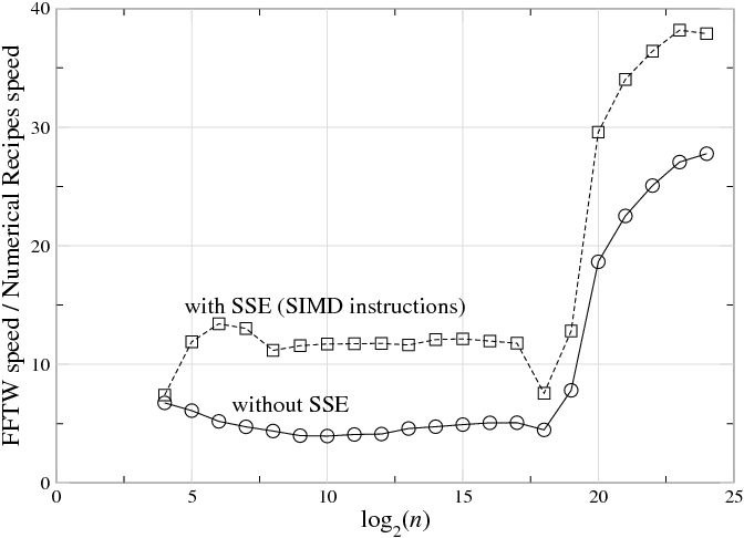
Fig. 10.1.1 The ratio of speed (1/time) between a highly optimized FFT (FFTW 3.1.2 ) and a typical textbook radix-2 implementation (Numerical Recipes in C on a 3 GHz Intel Core Duo with the Intel C compiler 9.1.043, for single-precision complex-data DFTs of size nn" role="presentation" style="position:relative;" tabindex="0">\(n\), plotted versus log2nlog2n" role="presentation" style="position:relative;" tabindex="0">\(\log _2n\). Top line (squares) shows FFTW with SSE SIMD instructions enabled, which perform multiple arithmetic operations at once (see section ); bottom line (circles) shows FFTW with SSE disabled, which thus requires a similar number of arithmetic instructions to the textbook code. (This is not intended as a criticism of Numerical Recipes—simple radix-2 implementations are reasonable for pedagogy—but it illustrates the radical differences between straightforward and optimized implementations of FFT algorithms, even with similar arithmetic costs.) For \(n\underset{\sim }{> }2^{19}\), the ratio increases because the textbook code becomes much slower (this happens when the DFT size exceeds the level-2 cache).
And yet there is a vast gap between this basic mathematical theory and the actual practice—highly optimized FFT packages are often an order of magnitude faster than the textbook subroutines, and the internal structure to achieve this performance is radically different from the typical textbook presentation of the “same” Cooley-Tukey algorithm. For example, Fig. 10.1.1 plots the ratio of benchmark speeds between a highly optimized FFT and a typical textbook radix-2 implementation, and the former is faster by a factor of 5–40 (with a larger ratio as nn" role="presentation" style="position:relative;" tabindex="0">n grows). Here, we will consider some of the reasons for this discrepancy, and some techniques that can be used to address the difficulties faced by a practical high-performance FFT implementation.2
In particular, in this chapter we will discuss some of the lessons learned and the strategies adopted in the FFTW library. FFTW is a widely used free-software library that computes the discrete Fourier transform (DFT) and its various special cases. Its performance is competitive even with manufacturer-optimized programs, and this performance is portable thanks the structure of the algorithms employed, self-optimization techniques, and highly optimized kernels (FFTW's codelets) generated by a special-purpose compiler.
This chapter is structured as follows. First Review of the Cooley-Tukey FFT we briefly review the basic ideas behind the Cooley-Tukey algorithm and define some common terminology, especially focusing on the many degrees of freedom that the abstract algorithm allows to implementations. Next, in Goals and Background of the FFTW Project we provide some context for FFTW's development and stress that performance, while it receives the most publicity, is not necessarily the most important consideration in the implementation of a library of this sort. Third, in FFTs and the Memory Hierarchy we consider a basic theoretical model of the computer memory hierarchy and its impact on FFT algorithm choices: quite general considerations push implementations towards large radices and explicitly recursive structure. Unfortunately, general considerations are not sufficient in themselves, so we will explain in Adaptive Composition of FFT Algorithms how FFTW self-optimizes for particular machines by selecting its algorithm at runtime from a composition of simple algorithmic steps. Furthermore, Generating Small FFT Kernels describes the utility and the principles of automatic code generation used to produce the highly optimized building blocks of this composition, FFTW's codelets. Finally, we will briefly consider an important non-performance issue, in Numerical Accuracy in FFTs.
Footnotes
1 We employ the standard asymptotic notation of \(O\) for asymptotic upper bounds, \(\Theta\) for asymptotic tight bounds, and \(\Omega\) for asymptotic lower bounds
2 We won't address the question of parallelization on multi-processor machines, which adds even greater difficulty to FFT implementation—although multi-processors are increasingly important, achieving good serial performance is a basic prerequisite for optimized parallel code, and is already hard enough!

