
1.6: An Electric Field Computation
- Page ID
- 9952

We have established that vectors may be used to code complex numbers. Conversely, complex numbers may be used to code or represent the orthogonal components of any two-dimensional vector. This makes them invaluable in electromagnetic field theory, where they are used to represent the components of electric and magnetic fields.
The basic problem in electromagnetic field theory is to determine the electric or magnetic field that is generated by a static or dynamic distribution of charge. The key idea is to isolate an infinitesimal charge, determine the field set up by this charge, and then to sum the fields contributed by all such infinitesimal charges. This idea is illustrated in Figure, where the charge \(λ\), uniformly distributed over a line segment of length \(dx\) at point \(−x\), produces a field \(dE(x)\) at the test point \((0,h)\). The field \(dE(x)\) is a “vector” field (as opposed to a “scalar” field), with components \(E1(x)\) and \(E2(x)\). The intensity or field strength of the field \(dE(x)\) is
\[|dE(x)|=\frac {λdx} {4πϵ_0(h^2+x^2)} \nonumber \]
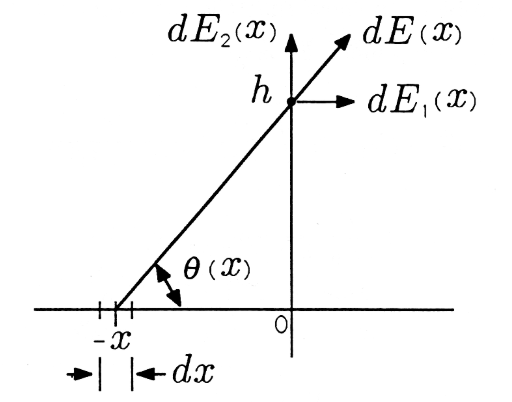
But the field strength is directed at angle \(θ(x)\), as illustrated in Figure. The field \(dE(x)\) is real with components \(dE_1(x)\) and \(dE_2(x)\), but we code it as a complex field. We say that the “complex” field at test point \((0,h)\) is
\[dE(x)=\frac {λdx} {4πϵ_0(h^2+x^2)} e^{jθ(x)} \nonumber \]
with components \(dE_1(x)\) and \(dE_2(x)\). That is,
\[dE(x)=dE_1(x)+jdE_2(x) \nonumber \]
\[dE_1(x)=\frac {λdx} {4πϵ_0(h^2+x^2)} \cosθ(x) \nonumber \]
\[dE_2(x)=\frac {λdx} {4πϵ_0(h^2+x^2)} \sinθ(x) \nonumber \]
For charge uniformally distributed with density \(λ\) along the x-axis, the total field at the test point \((0,h)\) is obtained by integrating \(dE\)
\[∫^∞_{−∞}dE(x)=∫^∞_{−∞} \frac {λ} {4πϵ_0(h^2+x^2)} [\cosθ(x)+j\sinθ(x)]dx \nonumber \]
The functions \(\cosθ(x)\) and \(\sinθ(x)\) are
\[\cosθ(x)=\frac {x} {(x^2+h^2)^{1/2}} ; \sinθ(x)=\frac {h} {(x^2+h^2)^{1/2}} \nonumber \]
We leave it as a problem to show that the real component \(E_1\) of the field is zero. The imaginary component \(E_2\) is
\[E=jE_2=j∫^∞_{−∞} \frac {λh} {4πϵ_0} \frac {dx} {(x^2+h^2)^{3/2}} \nonumber \]
\[=j\frac {λh} {4πϵ_0} \frac {x} {h^2(x^2+h^2)^{1/2}}∣^∞_{−∞} \nonumber \]
\[=j\frac {λh} {4πϵ_0} [\frac 1 {h^2} + \frac 1 {h_2}] = j\frac {λ} {2πϵ_0h} \nonumber \]
\[E_2=\frac λ {2πϵ_0h} \nonumber \]
We emphasize that the field at (0,h) is a real field. Our imaginary answer simply says that the real field is oriented in the vertical direction because we have used the imaginary part of the complex field to code the vertical component of the real field.
Show that the horizontal component of the field \(E\) is zero. Interpret this finding physically.
From the symmetry of this problem, we conclude that the field around the infinitely long wire of the Figure is radially symmetric. So, in polar coordinates, we could say
\[E(r,θ)=\frac λ {2πϵ_0r} \nonumber \]
which is independent of θ. If we integrated the field along a radial line perpendicular to the wire, we would measure the voltage difference
\[V(r_1)−V(r_0)=∫^{r_1}_{r_0}\frac λ {2πϵ_0r}dr=\frac λ {2πϵ_0}[\mathrm{log}r_1−\mathrm{log}r_0] \nonumber \]
An electric field has units of volts/meter, a charge density λ has units of coulombs/meter, and \(ϵ_0\) has units of coulombs/volt-meter; voltage has units of volts (of course).