
1: Introduction to Aerodynamics
- Page ID
- 75445

\( \newcommand{\vecs}[1]{\overset { \scriptstyle \rightharpoonup} {\mathbf{#1}} } \)
\( \newcommand{\vecd}[1]{\overset{-\!-\!\rightharpoonup}{\vphantom{a}\smash {#1}}} \)
\( \newcommand{\dsum}{\displaystyle\sum\limits} \)
\( \newcommand{\dint}{\displaystyle\int\limits} \)
\( \newcommand{\dlim}{\displaystyle\lim\limits} \)
\( \newcommand{\id}{\mathrm{id}}\) \( \newcommand{\Span}{\mathrm{span}}\)
( \newcommand{\kernel}{\mathrm{null}\,}\) \( \newcommand{\range}{\mathrm{range}\,}\)
\( \newcommand{\RealPart}{\mathrm{Re}}\) \( \newcommand{\ImaginaryPart}{\mathrm{Im}}\)
\( \newcommand{\Argument}{\mathrm{Arg}}\) \( \newcommand{\norm}[1]{\| #1 \|}\)
\( \newcommand{\inner}[2]{\langle #1, #2 \rangle}\)
\( \newcommand{\Span}{\mathrm{span}}\)
\( \newcommand{\id}{\mathrm{id}}\)
\( \newcommand{\Span}{\mathrm{span}}\)
\( \newcommand{\kernel}{\mathrm{null}\,}\)
\( \newcommand{\range}{\mathrm{range}\,}\)
\( \newcommand{\RealPart}{\mathrm{Re}}\)
\( \newcommand{\ImaginaryPart}{\mathrm{Im}}\)
\( \newcommand{\Argument}{\mathrm{Arg}}\)
\( \newcommand{\norm}[1]{\| #1 \|}\)
\( \newcommand{\inner}[2]{\langle #1, #2 \rangle}\)
\( \newcommand{\Span}{\mathrm{span}}\) \( \newcommand{\AA}{\unicode[.8,0]{x212B}}\)
\( \newcommand{\vectorA}[1]{\vec{#1}} % arrow\)
\( \newcommand{\vectorAt}[1]{\vec{\text{#1}}} % arrow\)
\( \newcommand{\vectorB}[1]{\overset { \scriptstyle \rightharpoonup} {\mathbf{#1}} } \)
\( \newcommand{\vectorC}[1]{\textbf{#1}} \)
\( \newcommand{\vectorD}[1]{\overrightarrow{#1}} \)
\( \newcommand{\vectorDt}[1]{\overrightarrow{\text{#1}}} \)
\( \newcommand{\vectE}[1]{\overset{-\!-\!\rightharpoonup}{\vphantom{a}\smash{\mathbf {#1}}}} \)
\( \newcommand{\vecs}[1]{\overset { \scriptstyle \rightharpoonup} {\mathbf{#1}} } \)
\(\newcommand{\longvect}{\overrightarrow}\)
\( \newcommand{\vecd}[1]{\overset{-\!-\!\rightharpoonup}{\vphantom{a}\smash {#1}}} \)
\(\newcommand{\avec}{\mathbf a}\) \(\newcommand{\bvec}{\mathbf b}\) \(\newcommand{\cvec}{\mathbf c}\) \(\newcommand{\dvec}{\mathbf d}\) \(\newcommand{\dtil}{\widetilde{\mathbf d}}\) \(\newcommand{\evec}{\mathbf e}\) \(\newcommand{\fvec}{\mathbf f}\) \(\newcommand{\nvec}{\mathbf n}\) \(\newcommand{\pvec}{\mathbf p}\) \(\newcommand{\qvec}{\mathbf q}\) \(\newcommand{\svec}{\mathbf s}\) \(\newcommand{\tvec}{\mathbf t}\) \(\newcommand{\uvec}{\mathbf u}\) \(\newcommand{\vvec}{\mathbf v}\) \(\newcommand{\wvec}{\mathbf w}\) \(\newcommand{\xvec}{\mathbf x}\) \(\newcommand{\yvec}{\mathbf y}\) \(\newcommand{\zvec}{\mathbf z}\) \(\newcommand{\rvec}{\mathbf r}\) \(\newcommand{\mvec}{\mathbf m}\) \(\newcommand{\zerovec}{\mathbf 0}\) \(\newcommand{\onevec}{\mathbf 1}\) \(\newcommand{\real}{\mathbb R}\) \(\newcommand{\twovec}[2]{\left[\begin{array}{r}#1 \\ #2 \end{array}\right]}\) \(\newcommand{\ctwovec}[2]{\left[\begin{array}{c}#1 \\ #2 \end{array}\right]}\) \(\newcommand{\threevec}[3]{\left[\begin{array}{r}#1 \\ #2 \\ #3 \end{array}\right]}\) \(\newcommand{\cthreevec}[3]{\left[\begin{array}{c}#1 \\ #2 \\ #3 \end{array}\right]}\) \(\newcommand{\fourvec}[4]{\left[\begin{array}{r}#1 \\ #2 \\ #3 \\ #4 \end{array}\right]}\) \(\newcommand{\cfourvec}[4]{\left[\begin{array}{c}#1 \\ #2 \\ #3 \\ #4 \end{array}\right]}\) \(\newcommand{\fivevec}[5]{\left[\begin{array}{r}#1 \\ #2 \\ #3 \\ #4 \\ #5 \\ \end{array}\right]}\) \(\newcommand{\cfivevec}[5]{\left[\begin{array}{c}#1 \\ #2 \\ #3 \\ #4 \\ #5 \\ \end{array}\right]}\) \(\newcommand{\mattwo}[4]{\left[\begin{array}{rr}#1 \amp #2 \\ #3 \amp #4 \\ \end{array}\right]}\) \(\newcommand{\laspan}[1]{\text{Span}\{#1\}}\) \(\newcommand{\bcal}{\cal B}\) \(\newcommand{\ccal}{\cal C}\) \(\newcommand{\scal}{\cal S}\) \(\newcommand{\wcal}{\cal W}\) \(\newcommand{\ecal}{\cal E}\) \(\newcommand{\coords}[2]{\left\{#1\right\}_{#2}}\) \(\newcommand{\gray}[1]{\color{gray}{#1}}\) \(\newcommand{\lgray}[1]{\color{lightgray}{#1}}\) \(\newcommand{\rank}{\operatorname{rank}}\) \(\newcommand{\row}{\text{Row}}\) \(\newcommand{\col}{\text{Col}}\) \(\renewcommand{\row}{\text{Row}}\) \(\newcommand{\nul}{\text{Nul}}\) \(\newcommand{\var}{\text{Var}}\) \(\newcommand{\corr}{\text{corr}}\) \(\newcommand{\len}[1]{\left|#1\right|}\) \(\newcommand{\bbar}{\overline{\bvec}}\) \(\newcommand{\bhat}{\widehat{\bvec}}\) \(\newcommand{\bperp}{\bvec^\perp}\) \(\newcommand{\xhat}{\widehat{\xvec}}\) \(\newcommand{\vhat}{\widehat{\vvec}}\) \(\newcommand{\uhat}{\widehat{\uvec}}\) \(\newcommand{\what}{\widehat{\wvec}}\) \(\newcommand{\Sighat}{\widehat{\Sigma}}\) \(\newcommand{\lt}{<}\) \(\newcommand{\gt}{>}\) \(\newcommand{\amp}{&}\) \(\definecolor{fillinmathshade}{gray}{0.9}\)Chapter 1. Introduction to Aerodynamics
1.1 Aerodynamics
Aerodynamics is probably the first subject that comes to mind when most people think of Aeronautical or Aerospace Engineering. Aerodynamics is essentially the application of classical theories of “fluid mechanics” to external flows or flows around bodies, and the main application which comes to mind for most aero engineers is flow around wings.
The wing is the most important part of an airplane because without it there would be no lift and no aircraft. Most people have some idea of how a wing works; that is, by making the flow over the top of the wing go faster than the flow over the bottom we get a lower pressure on the top than on the bottom and, as a result, get lift. The aero engineer needs to know something more than this. The aero engineer needs to know how to shape the wing to get the optimum combination of lift and drag and pitching moment for a particular airplane mission. In addition he or she needs to understand how the vehicle’s aerodynamics interacts with other aspects of its design and performance. It would also be nice if the forces on the wing did not exceed the load limit of the wing structure.
If one looks at enough airplanes, past and present, he or she will find a wide variety of wing shapes. Some aircraft have short, stubby wings (small wing span), while others have long, narrow wings. Some wings are swept and others are straight. Wings may have odd shapes at their tips or even attachments and extensions such as winglets. All of these shapes are related to the purpose and design of the aircraft.
In order to look at why wings are shaped like they are we need to start by looking at the terms that are used to define the shape of a wing.
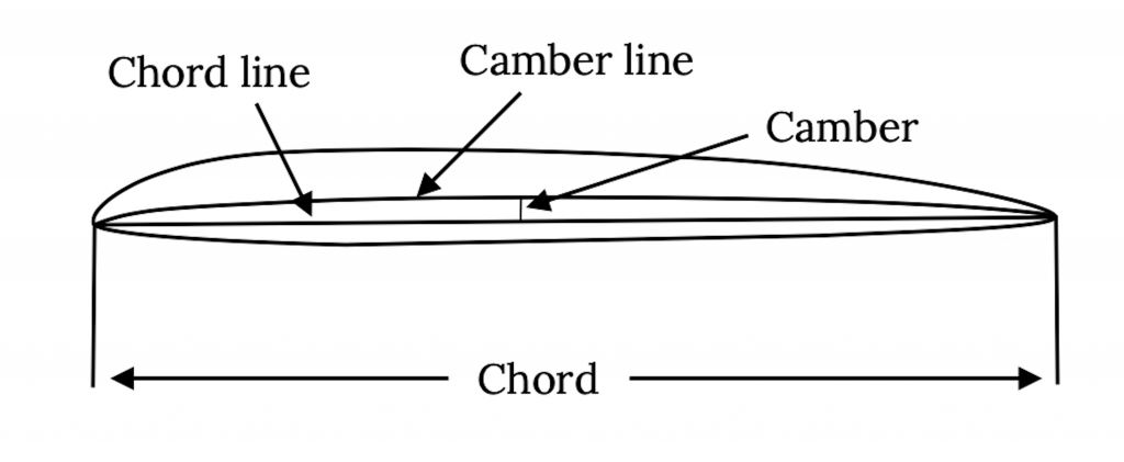
A two dimensional slice of a wing cut parallel to the centerline of the aircraft fuselage or body is called the airfoil section. A straight line from the airfoil section leading edge to its trailing edge is called the chord line. The length of the chord line is referred to as the chord. A line drawn half way between the airfoil section’s upper and lower surfaces is called the camber line. The maximum distance between the camber line and chord line is referred to as the airfoil’s camber and is usually enumerated as a percent of chord. We will see that the amount of airfoil camber and the location of the point of maximum camber are important numbers in defining the shape of an airfoil and predicting its performance. For most airfoils the maximum camber is on the order of zero to five percent and the location of the point of maximum camber is between 25% and 50% of the chord from the airfoil leading edge.
When viewed from above the aircraft the wing shape or planform is defined by other terms.
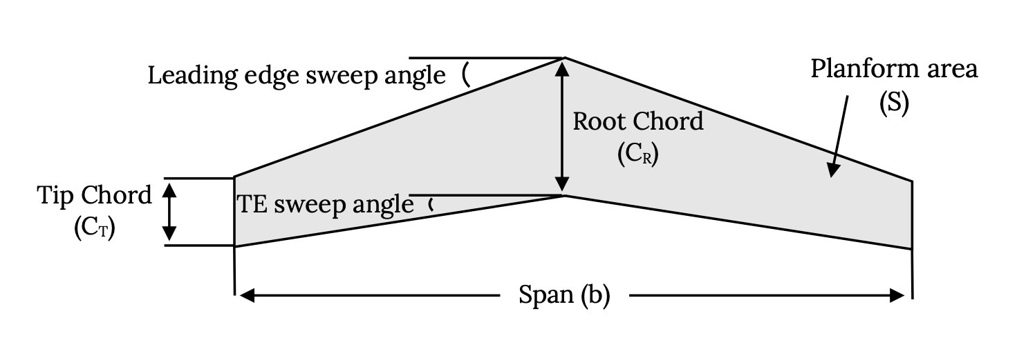
Note that the planform area is not the actual surface area of the wing but is “projected area” or the area of the wing’s shadow. Also note that some of the abbreviations used are not intuitive; the span, the distance from wing tip to wing tip (including any fuselage width) is denoted by b and the planform area is given a symbol of “S” rather than perhaps “A”. Sweep angles are usually given a symbol of lambda (λ).
Another definition that is based on the planform shape of a wing is the Aspect Ratio (AR).
AR = b2/S.
Aspect ratio is also the span divided by the “mean” or average chord. We will later find that aspect ratio is a measure of the wing’s efficiency in long range flight.
Wing planform shapes may vary considerably from one type of aircraft to another. Fighter aircraft tend to have low aspect ratio or short, stubby wings, while long range transport aircraft have higher aspect ratio wing shapes, and sailplanes have yet higher wing spans. Some wings are swept while others are not. Some wings have triangular or “delta” planforms. If one looks at the past 100 years of wing design he or she will see an almost infinite variety of shapes. Some of the shapes come from aerodynamic optimization while others are shaped for structural benefit. Some are shaped the way they are for stealth, others for maneuverability in aerobatic flight, and yet others just to satisfy their designer’s desire for a good looking airplane.
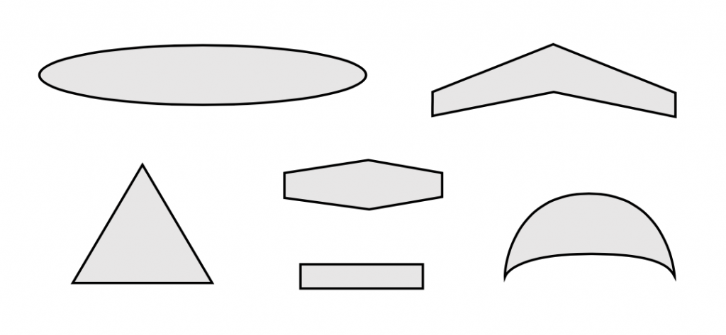
In general, high aspect ratio wings are desirable for long range aircraft while lower aspect ratio wings allow more rapid roll response when maneuverability is a requirement. Sweeping a wing either forward or aft will reduce its drag as the plane’s speed approaches the speed of sound but will also reduce its efficiency at lower speeds. Delta wings represent a way to get a combination of high sweep and a large area. Tapering a wing to give it lower chord at the wing tips usually gives somewhat better performance than an untapered wing and a non-linear taper which gives a “parabolic” planform will theoretically give the best performance.
In the following material we will take a closer look at some of the things mentioned above and at their consequences related to the flight capability of an airplane.
Before we take a more detailed look at wing aerodynamics we will first examine the atmosphere in which aircraft must operate and look at a few of the basic relationships we encounter in “doing” aerodynamics.
1.2 Air, Our Flight Environment
Airplanes operate in air, a gas made up of nitrogen, oxygen, and several other constituents. The behavior of air, that is the way its properties like temperature, pressure, and density relate to each other, can be described by the Ideal or Perfect Gas Equation of State:

where P is the barometric or hydrostatic pressure, ρ is the density, and T is the temperature. R is the gas constant for air. In this equation the temperature and pressure must be given in absolute values; in other words, temperature must be in Kelvin or Rankine, not Celsius (Centigrade) or Fahrenheit. Of course the units must all be consistent with those used in the gas constant:
1.3 Units
This brings us to the subject of units. It is important that all the units in the perfect gas equation be compatible; i.e., all English units or all SI units, and that we be careful if solving for, for example, pressure, to make sure that the units of pressure come out as they should (pounds per square foot in the English system or Pascals in SI). Unfortunately many of us don’t have a clue as to how to work with units.
It is popular in U. S. scientific circles to try to convince everyone that Americans are the only people in the world who use “English” units and the only people in the world who don’t know how to use SI units properly. Nothing could be further from the truth. No one in the world actually uses SI units correctly in everyday life. For example, the rest of the world commonly uses the Kilogram as a unit of weight when it is actually a unit of mass. They buy produce in the grocery store in Kilograms, not Newtons. You would also be hard pressed to find anyone in the world, even in France, who knows that a Pascal is a unit of pressure. Newtons and Pascals are simply not used in many places outside of textbooks. In England the distances on highways are still given in miles and speeds are given in mph even as the people measure shorter distances in meters (or metres), and the government is still trying to get people to stop weighing vegetables in pounds. There are many people in England who still give their weight in “stones”.
As aerospace engineers we will find that, despite what many of our textbooks say, most work in the industry is done in the English system, not SI, and some of it is not even done in proper English units. Airplane speeds are measured in miles per hour or in knots, and distances are often quoted in nautical miles. Pressures are given to pilots in inches of mercury or in millibars. Pressures inside jet and rocket engines are normally measured in pounds-per-square-inch (psi). Airplane altitudes are most often quoted in feet. Engine power is given in horsepower and thrust in pounds. We must be able to work in the real world, as well as in the politically correct world of the high school or college physics or chemistry or even engineering text.
It should be noted that what we in America refer to as the “English” unit system, people in England call “Imperial” units. This can get really confusing because “imperial” liquid measures are different from “American” liquid measures. An “imperial” gallon is slightly larger than an American gallon and a “pint” of beer in Britain is not the same size as a “pint” of beer in the U. S.
So, there are many possible systems of units in use in our world. These include the SI system, the pound-mass based English system, the “slug” based English system, the cgs-metric system, and others. We can discuss all of these in terms of a very familiar equation, Isaac Newton’s good old F = ma. Newton’s law relates units as well as physical properties and we can use it to look at several common unit systems.
Force = mass x acceleration
1 Newton = 1 kg x 1 meter/sec2
1 pound-force = 1 pound-mass x 32.17 ft/sec2
1 Dyne = 1 gram x 1 cm/sec2
1 pound-force = 1 slug x 1 ft/sec2
The first and last of the above are the systems with which we need to be thoroughly familiar; the first because it is the “ideal” system according to most in the scientific world, and the last because it is the semi-official system of the world of aerospace engineering.
In using any unit system there are three basic requirements:
- Always write units with any number that has units.
- Always work through the units in equations at the same time that you work out the numbers.
- Always reduce the final units to their simplest form and verify that they are the appropriate units for that number.
Following the above suggestions would eliminate about half of the wrong answers found on most student homework and test papers.
In doing engineering problems one should carry through the units as described above and make sure that the units make sense for the answer and that the magnitude of the answer is reasonable. Good students do this all the time while poor ones leave everything to chance.
The first part of this is simple. If the units in an answer don’t make sense, for example, if the speed for an airplane is calculated to be 345 feet per pound or if we calculate a weight to be 1500 kilograms per second, it should be easy to recognize that something is wrong. A fundamental error has been made in following through the problem with the units and this must be corrected.
The more difficult task is to recognize when the magnitude of an answer is wrong; i.e., is not “in the right ballpark”. If we are told that the speed of a car is 92 meters/sec. or is 125 ft/sec. do we have any “feel” for whether these are reasonable or not? Is this car speeding or not? Most of us don’t have a clue without doing some quick calculations (these are 205 mph and 85 mph, respectively). Do any of us know our weight in Newtons? What is a reasonable barometric pressure in the atmosphere in any unit system?
So our second unit related task is to develop some appreciation for the “normal” range of magnitudes for the things we want to calculate in our chosen units system(s). What is a reasonable range for a wing’s lift coefficient or drag coefficient? Is it reasonable for cars to have 10 times the drag coefficient of airplanes?
With these cautions in mind let’s go back and look at our “working medium”, the standard atmosphere.
1.4 The Standard Atmosphere
We said we were starting with the Ideal Gas Equation of State, P=RT. We will also make use of the Hydrostatic Equation, another relationship you have seen before in chemistry and physics:

This tells us how pressure changes with height in a column of fluid. This tells us how pressure changes as we move up or down through the atmosphere.
These two equations, the Perfect Gas Equation of State and the Hydrostatic Equation, have three variables in them; pressure, density, and temperature. To solve for these properties at any point in the atmosphere requires us to have one more equation, one involving temperature. This is going to require our first assumption. We must have some relationship that can tell us how temperature should vary with altitude in the atmosphere.
Many years of measurement and observation have shown that, in general, the lower portion of the atmosphere, where most airplanes fly, can be modeled in two segments, the Troposphere and the Stratosphere. The temperature in the troposphere is found to drop fairly linearly as altitude increases. This linear decrease in temperature continues up to about 36,000 feet (about 11,000 meters). Above this altitude the temperature is found to hold constant up to altitudes over 100,000 ft. This constant temperature region is the lower part of the Stratosphere. The troposphere and stratosphere are where airplanes operate, so we need to look at these in detail.
1.5 The Troposphere
We model the linear temperature drop with altitude in the troposphere with a simple equation:
Talt = Tsealevel – Lh
where “L” is called the “lapse rate”. From over a hundred years of measurements it has been found that a normal, average lapse rate is:
L = 3.56oR / 1000 ft = 6.5oK / 1000 meters .
This is often taught to pilots in a strange mixture of units as 1.98 degrees Centigrade per thousand feet!
The other thing we need is a value for the sea level temperature. Our model, also based on averages from years of measurement, uses the following sea level values for pressure, density, and temperature.


TSL = 288 oK = 520 oR
So, to find temperature at any point in the troposphere we use:
T (oR) = 520 – 3.56(h),
where h is the altitude in thousands of feet, or
T (oK) = 288 – 6.5 (h)
where h is the altitude in thousands of meters.
We need to stress at this point that this temperature model for the Troposphere is merely a model, but it is the model that everyone in the aviation and aerospace community has agreed to accept and use. The chance of ever going to the seashore and measuring a temperature of 59oF is slim and even if we find that temperature it will surely change within a few minutes. Likewise, if we were to send a thermometer up in a balloon on any given day the chance of finding a “lapse rate” equal to the one defined as “standard” is slim to none, and, during the passage of a weather front, we may even find that temperature increases rather than drops as we move to higher altitudes. Nonetheless, we will work with this model and perhaps later learn to make corrections for non-standard days.
Now, if we are willing to accept the model above for temperature change in the Troposphere, all we have to do is find relationships to tell how the other properties, pressure and density, change with altitude in the Troposphere. We start with the differential form of the hydrostatic equation and combine it with the Perfect Gas equation to eliminate the density term.

or,
g")
which is rearranged to give
dP/P = – (g/RT)dh.
Now we substitute in the lapse rate relationship for the temperature to get
dP/P = {g/[R(TSL-Lh)]}dh.
This is now a relationship with only one variable (P) on the left and only one (h) on the right. It can be integrated to give

In a similar manner we can get a relationship to find the density at any altitude in the troposphere
/LR")
So now we have equations to find pressure, density, and temperature at any altitude in the troposphere. Care has to be taken with units when using these equations. All temperatures must be in absolute values (Kelvin or Rankine instead of Celsius or Fahrenheit). The exponents in the pressure and density ratio equations must be unitless. Exponents cannot have units!
We can use these equations up to the top of the Troposphere, that is, up to 11,000 meters or 36,100 feet in altitude. Above that altitude is the Stratosphere where temperature is modeled as being constant up to roughly 100,000 feet.
1.6 The Stratosphere
We can use the temperature lapse rate equation result at 11,000 meters altitude to find the temperature in this part of the Stratosphere.
Tstratosphere = 216.5oK = 389.99oR = constant
The equations for determining the pressure and density in the constant temperature part of the stratosphere are different from those in the troposphere since temperature is constant. And, since temperature is constant both pressure and density vary in the same manner.
/RT")
The term on the right in the equation is “e” or 2.718, evaluated to the power shown, where h1 is the 11,000 meters or 36,100 ft (depending on the unit system used) and h2 is the altitude where the pressure or density is to be calculated. T is the temperature in the stratosphere.
Using the above equations we can find the pressure, temperature, or density anywhere an airplane might fly. It is common to tabulate this information into a standard atmosphere table. Most such tables also include the speed of sound and the air viscosity, both of which are functions of temperature. Tables in both SI and English units are given below.
Table 1.1: Standard Atmosphere in SI Units
| h (km) | T (degrees C) | a (m / sec) | Px10^(-4)(N/m^2 ) (pascals) | P (kg/m^3) | u x10^5 (kg/m sec) |
|---|---|---|---|---|---|
| 0 | 15 | 340 | 10.132 | 1.226 | 1.78 |
| 1 | 8.5 | 336 | 8.987 | 1.112 | 1.749 |
| 2 | 2 | 332 | 7.948 | 1.007 | 1.717 |
| 3 | -4.5 | 329 | 7.01 | 0.909 | 1.684 |
| 4 | -11 | 325 | 6.163 | 0.82 | 1.652 |
| 5 | -17.5 | 320 | 5.4 | 0.737 | 1.619 |
| 6 | -24 | 316 | 4.717 | 0.66 | 1.586 |
| 7 | -30.5 | 312 | 4.104 | 0.589 | 1.552 |
| 8 | -37 | 308 | 3.558 | 0.526 | 1.517 |
| 9 | -43.5 | 304 | 3.073 | 0.467 | 1.482 |
| 10 | -50 | 299 | 2.642 | 0.413 | 1.447 |
| 11 | -56.5 | 295 | 2.261 | 0.364 | 1.418 |
| 12 | -56.5 | 295 | 1.932 | 0.311 | 1.418 |
| 13 | -56.5 | 295 | 1.65 | 0.265 | 1.418 |
| 14 | -56.5 | 295 | 1.409 | 0.227 | 1.418 |
| 15 | -56.5 | 295 | 1.203 | 0.194 | 1.418 |
| 16 | -56.5 | 295 | 1.027 | 0.163 | 1.418 |
| 17 | -56.5 | 295 | 0.785 | 0.141 | 1.418 |
| 18 | -56.5 | 295 | 0.749 | 0.121 | 1.418 |
| 19 | -56.5 | 295 | 0.64 | 0.103 | 1.418 |
| 20 | -56.5 | 295 | 0.546 | 0.088 | 1.418 |
| 30 | -56.5 | 295 | 0.117 | 0.019 | 1.418 |
| 45 | 40 | 355 | 0.017 | 0.002 | 1.912 |
| 60 | 70.8 | 372 | 0.003 | 0.00039 | 2.047 |
| 75 | -10 | 325 | 0.0006 | 0.00008 | 1.667 |
Table 1.2: Standard Atmosphere in English Units
| h (ft) | T (degrees F) | a (ft/sec) | p (lb/ft^2) | p (slugs/ft^3) | u x 10^7 (sl/ft-sec) |
|---|---|---|---|---|---|
| 0 | 59 | 1117 | 2116.2 | 0.002378 | 3.719 |
| 1,000 | 57.44 | 1113 | 2040.9 | 0.00231 | 3.699 |
| 2,000 | 51.87 | 1109 | 1967.7 | 0.002242 | 3.679 |
| 3,000 | 48.31 | ll05 | 1896.7 | 0.002177 | 3.659 |
| 4,000 | 44.74 | ll02 | 1827.7 | 0.002112 | 3.639 |
| 5,000 | 41.18 | 1098 | 1760.8 | 0.002049 | 3.618 |
| 6,000 | 37.62 | 1094 | 1696 | 0.001988 | 3.598 |
| 7,000 | 34.05 | 1090 | 1633 | 0.001928 | 3.577 |
| 8,000 | 30.49 | 1086 | 1571.9 | 0.001869 | 3.557 |
| 9,000 | 26.92 | 1082 | 1512.9 | 0.001812 | 3.536 |
| 10,000 | 23.36 | 1078 | 1455.4 | 0.001756 | 3.515 |
| ll,000 | 19.8 | 1074 | 1399.8 | 0.001702 | 3.495 |
| 12,000 | 16.23 | 1070 | 1345.9 | 0.001649 | 3.474 |
| 13,000 | 12.67 | 1066 | 1293.7 | 0.001597 | 3.453 |
| 14,000 | 9.1 | 1062 | 1243.2 | 0.001546 | 3.432 |
| 15,000 | 5.54 | 1058 | 1194.3 | 0.001497 | 3.411 |
| 16,000 | 1.98 | 1054 | 1147 | 0.001448 | 3.39 |
| 17,000 | -1.59 | 1050 | 1101.1 | 0.001401 | 3.369 |
| 18,000 | -5.15 | 1046 | 1056.9 | 0.001355 | 3.347 |
| 19,000 | -8.72 | 1041 | 1014 | 0.001311 | 3.326 |
| 20,000 | -12.28 | 1037 | 972.6 | 0.001267 | 3.305 |
| 21,000 | -15.84 | 1033 | 932.5 | 0.001225 | 3.283 |
| 22,000 | -19.41 | 1029 | 893.8 | 0.001183 | 3.262 |
| 23,000 | -22.97 | 1025 | 856.4 | 0.001143 | 3.24 |
| 24,000 | -26.54 | 1021 | 820.3 | 0.001104 | 3.218 |
| 25,000 | -30.1 | 1017 | 785.3 | 0.001066 | 3.196 |
| 26,000 | -33.66 | 1012 | 751.7 | 0.001029 | 3.174 |
| 27,000 | -37.23 | 1008 | 719.2 | 0.000993 | 3.153 |
| 28,000 | -40.79 | 1004 | 687.9 | 0.000957 | 3.13 |
| 29,000 | -44.36 | 999 | 657.6 | 0.000923 | 3.108 |
| 30,000 | -47.92 | 995 | 628.5 | 0.00089 | 3.086 |
| 31,000 | -51.48 | 991 | 600.4 | 0.000858 | 3.064 |
| 32,000 | -55.05 | 987 | 573.3 | 0.000826 | 3.041 |
| 33,000 | -58.61 | 982 | 547.3 | 0.000796 | 3.019 |
| 34,000 | -62.18 | 978 | 522.2 | 0.000766 | 2.997 |
| 35,000 | -65.74 | 973 | 498 | 0.000737 | 2.974 |
| 40,000 | -67.6 | 971 | 391.8 | 0.0005857 | 2.961 |
| 45,000 | -67.6 | 971 | 308 | 0.0004605 | 2.961 |
| 50,000 | -67.6 | 971 | 242.2 | 0.0003622 | 2.961 |
Table 1.2: Standard Atmosphere in English Units (con’t)
| h (ft) | T (degrees F) | a (ft/sec) | p (lb/ft^2) | p (slugs/ft^3) | u x 10^7(sl/ft-sec) |
|---|---|---|---|---|---|
| 60,000 | -67.6 | 971 | 150.9 | 0.000224 | 2.961 |
| 70,000 | -67.6 | 971 | 93.5 | 0.0001389 | 2.961 |
| 80,000 | -67.6 | 971 | 58 | 0.0000861 | 2.961 |
| 90,000 | -67.6 | 971 | 36 | 0.0000535 | 2.961 |
| 100,000 | -67.6 | 971 | 22.4 | 0.0000331 | 2.961 |
| 150,000 | 113.5 | 1174 | 3.003 | 0.00000305 | 4.032 |
| 200,000 | 159.4 | 1220 | 0.6645 | 0.00000062 | 4.277 |
| 250,000 | -8.2 | 1042 | 0.1139 | 0.00000015 | 3.333 |
A look at these tables will show a couple of terms that we have not discussed. These are the speed of sound “a”, and viscosity “μ”. The speed of sound is a function of temperature and decreases as temperature decreases in the Troposphere. Viscosity is also a function of temperature.
The speed of sound is a measure of the “compressibility” of a fluid. Water is fairly incompressible but air can be compressed as it might be in a piston/cylinder system. The speed of sound is essentially a measure of how fast a sound or compression wave can move through a fluid. We often talk about the speeds of high speed aircraft in terms of Mach number where Mach number is the relationship between the speed of flight and the speed of sound. As we get closer to the speed of sound (Mach One) the air becomes more compressible and it becomes more meaningful to write many equations that describe the flow in terms of Mach number rather than in terms of speed.
Viscosity is a measure of the degree to which molecules of the fluid bump into each other and transfer forces on a microscopic level. This becomes a measure of “friction” within a fluid and is an important term when looking at friction drag, the drag due to shear forces that occur when a fluid (air in our case) moves over the surface of a wing or body in the flow.
Two things should be noted in these tables about viscosity. First, the units look sort of strange. Second, the viscosity column is headed with μ X 10x. The units are the proper ones for viscosity in the SI and English systems respectively; however, if you talk to a chemist or physicist about viscosity they will probably quote numbers with units of “poise”. The 10xnumber in the column heading means that the number shown in the column has been multiplied by 10xto give it the value shown. This is, to most of us, not intuitive. What this means is that in the English unit version of the Standard Atmosphere table, the viscosity at sea level has a value of 3.719 times ten to the minus 7.
So now we can find the properties of air at any altitude in our model or “standard” atmosphere. However, this is just a model, and it would be rare indeed to find a day when the atmosphere actually matches our model. Just how useful is this?
In reality this model is pretty good when it comes to pressure variation in the atmosphere because it is based on the hydrostatic equation which is physically correct. On the other hand, pressure at sea level does vary from day to day with weather changes, as the area of concern comes under the various high or low pressure systems often noted on weather maps. Temperature represents the greatest opportunity for variation between the model and the real atmosphere, after all, how many days a year is the temperature at the beach 59oF (520oR)? Density, of course, is a function of pressure and temperature, so its “correctness” is dependent on that of P and T.
On the face of things, it appears that the Standard Atmosphere is somewhat of a fantasy. On the other hand, it does give us a pretty good idea of how these properties of air should normally change with altitude. And, we can possibly make corrections to answers found when using this model by correcting for actual sea level pressure and temperature if needed. Further, we could define other “standard” atmospheres if we are looking at flight conditions where conditions are exceptionally different from this model. This is done to give “Arctic Minimum” and “Tropical Maximum” atmosphere models.
In the end, we do all aircraft performance and aerodynamic calculations based on the normal standard atmosphere and all flight testing is done at standard atmosphere pressure conditions to define altitudes. The standard atmosphere is our model and it turns out that this model serves us well.
One way we use this model is to determine our altitude in flight.
1.7 Altitude Measurement
The pilot of an aircraft needs to know its altitude and there are several ways we could measure the altitude of an airplane. Radar might be used to measure the plane’s distance above the ground. Global Positioning System satellite signals can determine the plane’s position, including its altitude, in three dimensional space. These and some other possible methods of altitude determination depend on the operation of one or more electrical systems, and while we may want to have such an instrument on our airplane, we also are required to have an “altimeter” that does not depend on batteries or generators for its operation. Further, the altitude that the pilot needs to know is the height above sea level. The obvious solution is to use our knowledge that the pressure varies in a fairly dependable fashion with altitude.
If we know how pressure varies with altitude then we can measure that pressure and determine the altitude above a sea level reference point. In other words, if we measure the pressure as 836 pounds per square foot we can look in the standard atmosphere table and find that we should be at an altitude of 23,000 ft. So all we need to do is build a simple mechanical barometer and calibrate its dial so it reads in units of altitude rather than pressure. As the measured pressure decreases, the indicated altitude increases in accord with the standard atmosphere model. This is, in fact, how “simple” altimeters such as those sometimes used in cars or bikes or even “ultra-lite” aircraft. A barometer measures the air pressure and on some type of dial or scale, instead of pressure units, the equivalent altitudes are indicated.
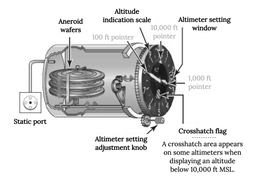
The “simple” altimeter, however, might not be quite accurate enough for most flying because of the variations in atmospheric pressure with weather system changes. The simple altimeter would base its reading on the assumption that the pressure at sea level is 2116 psf . If, however, we are in an area of “high” pressure, the altimeter of an airplane sitting at sea level would sense the higher than standard pressure and indicate an altitude somewhat below sea level. Conversely, in the vicinity of a low pressure atmospheric system the altimeter would read an altitude higher than the actual value. If this error was only a few feet it might not matter, but in reality it could result in errors of several hundred feet in altitude readings. This could lead to disaster in bad weather when a pilot has to rely on the altimeter to ensure that the plane clears mountain peaks or approaches the runway at the right altitude. Hence, all aircraft today use “sensitive” altimeters that allow the pilot to adjust the instrument for changes in pressure due to atmospheric weather patterns.
The sensitive altimeter, shown in the next figure, has a knob that can be turned to adjust the readout of the instrument for non-standard sea level pressures. This can be used in two different ways in flight. When the aircraft is sitting on the ground at an airport the pilot can simply adjust the knob until the altimeter reads the known altitude of the airport. In flight, the pilot can listen to weather report updates from nearby airports, reports that will include the current sea level equivalent barometric pressure, and turn the knob until the numbers in a small window on the altimeter face agree with the stated pressure. These readings are usually given in units of millimeters of mercury where 29.92 is sea level standard. Adjusting the reading in the window to a higher pressure will result in a decrease in the altimeter reading and adjusting it lower will increase the altitude indication. With proper and timely use of this adjustment a good altimeter should be accurate within about 50 feet.
It should be noted that we could also use density to define our altitude and, in fact, this might prove more meaningful in terms of relating to changes in an airplane’s performance at various flight altitudes because engine thrust and power are known to be functions of density and the aerodynamic lift and drag are also functions of density. However, to “measure” density would require measurement of both pressure and temperature. This could introduce more error into our use of the standard atmosphere for altitude determination than the use of pressure alone because temperature variation is much more subject to non-standard behavior than that of pressure. On the other hand, we do sometimes find it valuable to calculate our “density altitude” when looking at a plane’s ability to take-off in a given ground distance.
If we are at an airport which is at an altitude of, lets say, 4000 ft and the temperature is higher than the 44.74oF predicted by the standard atmosphere (as it probably would be in the summer) we would find that the airplane behaves as if it is at a higher altitude and will take a longer distance to become airborne than it should at 4000 ft. Pilots use either a circular slide rule type calculator or a special electronic calculator to take the measured real temperature and combine it with the pressure altitude to find the “density altitude”, and this can be used to estimate the extra takeoff distance needed relative to standard conditions.
Some may wonder why we can’t simply use temperature to find our altitude. After all, wasn’t one of our basic assumptions that in the Troposphere, temperature dropped linearly with altitude? Wouldn’t it be really easy to stick a thermometer out the window and compare its reading with a standard atmosphere chart to find our altitude?
Of course, once we are above the Troposphere this wouldn’t do any good since the temperature becomes constant over thousands of feet of altitude, but why wouldn’t it work in the Troposphere?
Thought Exercise
- Think about and discuss why using temperature to find altitude is not a good idea.
- Why is pressure the best property to measure to find our altitude?
- Perhaps using density to find altitude would be a better idea since density has a direct effect on flight performance. Think of one reason why we don’t have altimeters that measure air density.
1.8 Bernoulli’s Equation
You have undoubtedly been introduced to a relationship called Bernoulli’s Equation or the Bernoulli Principle somewhere in a previous Physics or Chemistry course. This is the principle that relates the pressure to the velocity in any fluid, essentially showing that as the speed of a fluid increases its pressure decreases and visa versa. This principle can take several different mathematical forms depending on the fluid and its speed. For an incompressible fluid such as water or for air below about 75% of the speed of sound this relationship takes the following form:
P + ½ρV2 = P0
(hydro)static pressure + dynamic pressure = total pressure
[internal energy + kinetic energy = total energy]
This relationship can be thought of as either a measure of the balance of pressure forces in a flow, or as an energy balance (first law of thermodynamics) when there is no change in potential energy or heat transfer.
Bernoulli’s equation says that along any continuous path (“streamline”) in a flow the total pressure, P0, (or total energy) is conserved (constant) and is a sum of the static pressure and the dynamic pressure in the flow. Static pressure and dynamic pressure can both change, but they must change in such a way that their sum is constant; i.e., as the flow speeds up the pressure decreases.
* ASSUMPTIONS: It is very important that we know and understand the assumptions that limit the use of this form of Bernoulli’s equation. The equation can be derived from either the first law of thermodynamics (energy conservation) or from a balance of forces in a fluid through what is known as Euler’s Equation. In deriving the form of the equation above some assumptions are made in order to make some of the math simpler. These involve things like assuming that density is a constant, making it a constant in an integration step in the derivation and making the integration easier. It is also assumed that mass is conserved, a seemingly logical assumption, but one that has certain consequences in the use of the equation. It is also assumed that the flow is “steady”, that is, the speed at any point in the flow is not varying with time. Another way to put this is that the speed can vary with position in the flow (that’s really what the equation is all about) but cannot vary with time.
The assumption of constant density, which we usually call an assumption of incompressible flow, means that we have to observe a speed limit. As air speeds up and the speed approaches the speed of sound its density changes; i.e., it becomes compressible. So when our flow speeds get too near the speed of sound, the incompressible flow assumption is violated and we can no longer use this form of Bernoulli’s equation. When does that become a problem?
Some fluid mechanics textbooks use a mathematical series relationship to look at the relationship between speed or Mach number (Mach number, the speed divided by the speed of sound, is really a better measure of compressibility than speed alone) and they use this to show that the incompressible flow assumption is not valid above a Mach number of about 0.3 or 0.3 times the speed of sound. This is good math but not so good physics. The important thing is not how the math works but how the relationship between the two pressures in Bernoulli’s equation changes as speed or Mach number increases. We will examine this in a later example to show that we are actually pretty safe in using the incompressible form of Bernoulli’s equation up to something like 75% of the speed of sound.
The other important assumptions in this form of Bernoulli’s equation are those of steady flow and mass conservation. Steady flow means pretty much what it sounds like; the equation is only able to account for changes in speed and pressure with position in a flow field. It was assumed that the flow is exactly the same at any time.
The mass conservation assumption really relates to looking at what are called “streamlines” in a flow. These can be thought of at a basic level as flow paths or highways that follow or outline the movement of the flow. Mass conservation implies that at any point along those paths or between any two streamlines the mass flow between the streamlines (in the path) is the same as it is at any other point between the same two streamlines (or along the same path).
The end result of this mass conservation assumption is that Bernoulli’s equation is only guaranteed to hold true along a streamline or path in a flow. However, we can extend the use of the relationship to any point in the flow if all the flow along all the streamlines (or paths) at some reference point upstream (at “∞”) has the same total energy or total pressure.
So, we can use Bernoulli’s equation to explain how a wing can produce lift. If the flow over the top of the wing is faster than that over the bottom, the pressure on the top will be less than that on the bottom and the resulting pressure difference will produce a lift. The study of aerodynamics is really all about predicting such changes in velocity and pressure around various shapes of wings and bodies. Aerodynamicists write equations to describe the way air speeds change around prescribed shapes and then combine these with Bernoulli’s equation to find the resulting pressures and forces.
Let’s look at the use of Bernoulli’s equation for the case shown below of a wing moving through the air at 100 meters/sec. at an altitude of 1km.
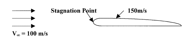
We want to find the pressure at the leading edge of the wing where the flow comes to rest (the stagnation point) and at a point over the wing where the speed has accelerated to 150 m/s.
First, note that the case of the wing moving through the air has been portrayed as one of a stationary wing with the air moving past it at the desired speed. This is standard procedure in working aerodynamics problems and it can be shown that the answers one finds using this method are the correct ones. Essentially, since the process of using Bernoulli’s equation is one of looking at conservation of energy, it doesn’t matter whether we are analyzing the motion (kinetic energy) involved as being motion of the body or motion of the fluid.
Now let’s think about the problem presented above. We know something about the flow at three points:
Well in front of the wing we have what is called “free stream” or undisturbed, uniform flow. We designate properties in this flow with an infinity [∞] subscript. We can write Bernoulli’s equation here as:
ρV∞2=P0whereV∞=100m/s")
Note that it is at this point, the “free stream” where all the flow is uniform and has the same total energy. If at this point the flow was not uniform, perhaps because it was near the ground and the speed increases with distance up from the ground, we could not assume that each “streamline” had a different value of total pressure (energy).
At the front of the wing we will have a point where the flow will come to rest. We call this point the “stagnation point” if we can assume that the flow slowed down and stopped without significant losses. Here the flow speed would be zero. We can write Bernoulli’s equation here as:
Pstagnation + 0 = P0
At this point the flow has accelerated to 150 m/s and we can write Bernoulli’s equation as:
ρV32=P0whereV3=150m/s")
Now we know that since the flow over the wing is continuous (mass is conserved) the total pressure (P0) is the same at all three points and this is what we use to find the missing information. To do this we must understand which of these pressures (if any) are known to us as atmospheric hydrostatic pressures and understand that we can assume that the density is constant as long as we are safely below the speed of sound.
Initially we know that the pressure in the atmosphere is that in the standard atmosphere table for an altitude of 1 km or 89870 Pascals and that the density at this altitude is 1.112 kg/m3. Looking at the problem, the most logical place for standard atmosphere conditions to apply is in the “free stream” location because this is where the undisturbed flow exists. Hence

And, using these in Bernoulli’s equation at the free stream location we calculate a total pressure
P0 = 95430 Pa
Now that we have found the total pressure we can use it at any other location in the flow to find the other unknown properties.
At the stagnation point
Pstagnation = P0 = 95430 Pa
At the point where the speed is 150 m/s we can rearrange Bernoulli’s equation to find
ρV32=82920Pa")
As a check we should confirm that the static pressure (P3) at this point is less than the free stream static pressure (P) since the speed is higher here and also confirm that the static pressures everywhere else in the flow are lower than the stagnation pressure.
Now let’s review the steps in working any problem with Bernoulli’s equation. First we must sketch the flow and write down everything we know at various points in that flow. Second we must write Bernoulli’s equation at every point in the flow where we either know information or want to know something. Third we must carefully assess which pressure, if any, can be obtained from the standard atmosphere table. Fourth we must look at all these points in the flow and see which point gives us enough information to solve for the total pressure (P0). Finally we use this value of P0 in Bernoulli’s equation at other points in the flow to find the other missing terms. Attempting to skip any of the above steps can lead to mistakes for most of us.
One of the most common problems that people have in working with Bernoulli’s equation in a problem like the one above is to assume that the stagnation point is the place to start the solution of the problem. They look at the three points in the flow and assume that the stagnation point must be the place where everything is known. After all, isn’t the velocity at the stagnation point equal to zero? Doesn’t this mean that the static pressure and the total pressure are the same here? And what other conclusion can be drawn than to assume that this pressure must then be the atmospheric pressure?
Well, the answer to the first two questions is “yes” but a third “yes” does not follow. What is known at the stagnation point is that the static pressure term in the equation is now the static pressure at a stagnation point and is therefore called the stagnation pressure. And, since the speed is zero, the stagnation pressure is equal to the total pressure in the flow. Neither of these pressures, however, is the atmospheric pressure.
Why is the pressure at the stagnation point not the pressure in the atmosphere? Well, this is where our substitution of a moving flow and a stationary wing for a moving wing in a stationary fluid ends up causing us some confusion. In reality, this stagnation point is where the wing is colliding head-on with the air that it is rushing through. The pressure here, the stagnation pressure, must be equal to the pressure in the atmosphere plus the pressure caused by the collision between wing and fluid; i.e., it must be higher than the atmospheric pressure.
Our approach of modeling the flow of a wing moving through the stationary atmosphere as a moving flow around a stationary wing makes it easier to work with Bernoulli’s equation in general; however, we must keep in mind that it is a substitute model and alter our way of looking at it appropriately. In this model the hydrostatic pressure is not the pressure where the air is “static”, it is, rather, the pressure where the flow is “undisturbed”. This is at the “free stream” conditions, the point upstream of the body (wing, in this case) where the flow has not yet felt the presence of the wing. This is where the undisturbed atmosphere exists. Between that point and the wing itself the flow has to change direction and speed as it moves around the body, so nowhere else in the flow field will the pressure be the same as in the undisturbed atmosphere.
1.9 Airspeed Measurement
Now that we know something about Bernoulli’s equation we can look at another use of the relationship, the measurement of airspeed. Rearranging the equation we can write:
/ρ]1/2")
So, if we know the total and static pressures at a point and the density at that point we can easily find the speed at that point. All we need is some way to measure or otherwise find these quantities.
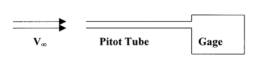
We can find the total pressure (P0) by simply inserting an open tube of some kind into the flow so that it is pointed into the oncoming flow and then connected to a pressure gage of some sort.
The static pressure can be found in a similar manner but the flow must be going parallel to the openings in the tube or surface.

On an airplane we usually mount a pitot tube somewhere on the wing or nose of the aircraft where it will generally point into the undisturbed flow and not be behind a propeller. The static pressure reading on an airplane is normally taken via a hole placed at some point on the side of the airplane where the flow will have the same static pressure as the freestream flow instead of using a separate static probe. This point is usually determined in flight testing. There is usually a static port on both sides of the plane connected to a single tube through a “T” connection. The static port looks like a small, circular plate with a hole in its center. One of the jobs required of the pilot in his or her preflight inspection of the aircraft is to make sure that both the pitot tube and static ports are free of obstruction, a particularly important task in the Spring of the year when insects like to crawl into small holes and build nests.
In a wind tunnel and in other experimental applications we often use a single instrument to measure both total and static pressures. This instrument is called a pitot-static tube and it is merely a combination of the two probes shown above.
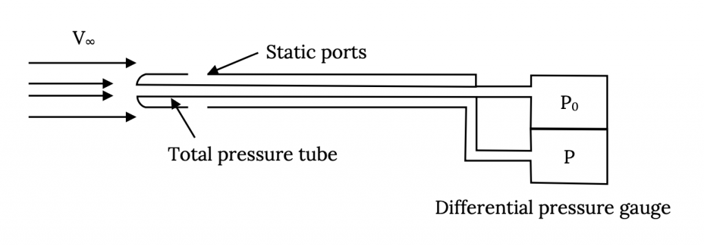
In both the lab case and the aircraft case it is the difference in the two pressures, P0 – P, that we want to know and this can be measured with several different types of devices ranging from a “U-tube” liquid manometer to a sophisticated electronic gage. In an aircraft, where we don’t want our knowledge of airspeed to depend on a source of electricity and where a liquid manometer would be cumbersome, the pressure difference is measured by a mechanical device called an aneroid barometer.
But let’s go back and look at the equation used to find the velocity and see if this causes any problem.
This shows that we also need to know the density if we wish to find the speed. In the lab we find the density easily enough by measuring the barometric pressure and the temperature and calculating density using the Ideal Gas Law,
or,

and, using this we can find the exact or “true” airspeed.
In an airplane we want simplicity and reliability, and while we could ask the pilot or some flight computer to measure pressure and temperature, then calculate density, then put it into Bernoulli’s equation to calculate airspeed, this seems a little burdensome and, of course, the use of computers or calculators might depend on electricity. Hence, we do not usually have an instrument on an aircraft that displays the true airspeed; instead we choose to simply measure the difference in the two above pressures using a mechanical instrument and then calibrate that instrument to display what we call the indicated airspeed, a measurement of speed based on the assumption of sea level density.
/ρSL]1/2")
Another name for the indicated airspeed is the “sea level equivalent airspeed”, the speed which would exist for the measured difference in static and total pressure if the aircraft was at sea level.
The true and indicated airspeeds are directly related by the square root of the ratio of sea level and true densities.

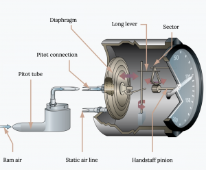
The airspeed indicator on an aircraft then measures the indicated airspeed and not the true airspeed. It is a sealed instrument with the static pressure going to the instrument container and the total pressure connected to an aneroid barometer inside the container. As the difference in these two pressures changes, the indicator needles on the instrument face move over a dial marked off, not for a range of pressures, but for a range of speeds. Each such instrument is carefully calibrated to ensure accurate measurement of indicated airspeed.
So, just as we found that the altimeter on an airplane measures the wrong altitude unless we are able to adjust it properly, the airspeed indicator does not measure the real airspeed. Is this a problem for us?
It turns out that, as far as the performance of the aircraft is concerned; i.e., its ability to take off in a certain distance, to climb at a certain rate, etc., is actually dependent on the indicated airspeed rather than the true airspeed. Yes, we want to know the true airspeed to know how fast we are really going and for related flight planning purposes, but as far as knowing the speed at which to rotate on takeoff, the best speed at which to climb or glide, and so on, we are better off using the indicated airspeed.
The indicated airspeed, since the density is assumed to always be sea level conditions, is really a function only of the difference in total and static pressures, P0 – P, which we know from Bernoulli’s equation is equal to:
and we are going to find that the terms on the right, the dynamic pressure, is a very important term in accounting for the forces on a body in a fluid. In other words, the plane’s behavior in flight is much more dependent on the dynamic pressure than on the airspeed alone.
Example: Let’s look at the difference between true and indicated airspeed just to get some idea of how big this difference might be. Lets pick an altitude of 15,000 feet and see what the two values of airspeed would be if the pitot-static system is exposed to a pressure difference of 300 pounds-per-square-foot (psf). The density in the standard atmosphere for 15,000 feet is 0.001497 sl/ft3 while that at sea level is 0.002378 sl/ft3.
/ρSL]1/2=502ft/sec")

So the difference in these two readings can be significant, but that is OK. We use the indicated airspeed to fly the airplane and use the true airspeed when finding the time for the trip. Note that when working Bernoulli’s equation problems, such as in finding the variations in pressures and velocity around a wing, you always want to use the true airspeed and the real pressures and density at altitude.
Finally, while on the subject of airspeed, we should note that even though we often calculate the speed of an aircraft or wing in units of feet/sec. or meters/sec., most airspeed indicators will show the airspeed in units of either miles-per-hour or knots. The knot is a rather ancient unit of speed used for centuries by sailors and once measured by timing a knotted rope as it was lowered over the side of a ship into the flowing sea.
A knot is a nautical-mile-per-hour and a nautical mile is a set fraction of the earth’s circumference. In relationship to more familiar English units:
1 knot (kt) = 1.15 mph
1 nautical mile (nm) = 1.15 “statute” miles (mi).
It is common practice in all parts of the world for our politically correct unit systems to be totally ignored and to do all flight planning and flying using units of knots and nautical miles for speed and distance.
1.10 Bernoulli’s Equation for Compressible Flow
The form of Bernoulli’s equation that we have been using is for incompressible flow as has been noted several times. What if the flow isn’t incompressible?
If Bernoulli’s equation was derived without making the assumption of constant air density it would come out in a different form and would be a relationship between pressures and Mach number. The relationship would also have another parameter in it, a term called gamma (γ). Gamma is simply a number for a given gas and the number depends on the number of atoms in the gas molecule, whether it is monatomic or diatomic, etc. Air is really a mixture of gasses but, in general, it is considered a diatomic gas. Its value of gamma is 1.4.
[Another name for gamma is the “ratio of specific heats” or the specific heat at constant pressure divided by the specific heat at constant density. These specific heats are a measure of the way heat is transferred in a gas under certain constraints (constant pressure or density) and this is, in turn, dependent on the molecular composition of the gas. In some other fields, Thermodynamics for example, the letter “k” is used for this ratio instead of γ.]
When a flow must be considered compressible this relationship between pressures and speed or Mach number takes the form below:
(P0/P) = {1 + [(γ-1)/2]M2 }[(γ-1)/(γ)]
If you use both this equation and the incompressible form of Bernoulli’s equation to solve for total pressure for given speeds from zero to 1000 ft/sec., using sea level conditions and the speed of sound at sea level to find the Mach number associated with each speed, and then compare the compressible and incompressible values of the total pressure (P0) you will find just over 2% difference at 700 ft/sec. and 5% at 900 ft/sec. In other words, the use of Bernoulli’s incompressible equation to find pressure and speed relationships is pretty reasonable up to speeds of about 75% of the speed of sound!
1.11 Forces in a Fluid
Above it was noted that the behavior of an airplane in flight is dependent on the dynamic pressure rather than on speed or velocity alone. In other words, it is a certain combination of density and velocity and not just density or velocity alone that is important to the way an airplane or a rocket flies. A question that might be asked is if there are other combinations of fluid properties that also have a major influence on aerodynamic forces.
We have already looked at one of these, Mach number, a combination of the speed and the speed of sound. Why is Mach number a “unique” combination of properties? Are there others that are just as important?
There is a fairly simple way we can take a look at how such combinations of fluid flow parameters group together to influence the forces and moments on a body in that flow. In more sophisticated texts this is found through a process known as “dimensional analysis”, and in books where the author was more intent on demonstrating his mathematical prowess than in teaching an understanding of physical reality, the process uses something called the “Buckingham-Pi Theorem”. Here, we will just be content with a description of the simplest process.
If we look at the properties in a fluid and elsewhere that cause forces on a body like an airplane in flight we could easily name several things like density, pressure, the size of the body, gravity, the “stickiness” or “viscosity” of the fluid and so on. As it turns out we could fairly easily say that most forces on an aircraft or rocket in flight are in some way functions of the following things:
")
where,
ρ = density
V = velocity
l = a representative length or size of the body
μ = viscosity
P = pressure
g = gravity (weight)
a = speed of sound
Viscosity must be considered to account for friction between the flow and the body and the speed of sound is included because somewhere we have heard that there are things like large drag increases at speeds near the speed of sound.
We really don’t know at this point exactly how general to be in looking at these terms. For example, we already know from Bernoulli’s equation that it is velocity squared that is important and not just velocity, at least in some cases. And, we might expect that instead of length it is length squared (area) that is important in the production of forces since we know forces come from a pressure acting on an area. So let’s be completely general and say the following:
")
Our simple analysis does not seek to find exact relationships or numbers but only the correct functional dependencies or combination of parameters. The analysis is really just a matter of balancing the units on the two sides of the equation. On the left side we have units of force (pounds or Newtons) where we know that one pound is equal to one slug times one ft/sec.2 or that one Newton is a kilogram-meter per second2. So the combination of all the units inherent in all the terms on the right side of the equation must also come out in these exact same unit combination as found on the left side of the equation. In other words, when all the units are accounted for on the right hand side of the equation the must combine to have units of force;
(sl)1(ft)1(sec)-2 or (mass)1(length)1(time)-2.
So, in this game of dimensional analysis the procedure is to replace each physical term on both sides of the equation with its proper units. Then we can simply add up all the exponents on both sides and write equations relating unit powers. For example, on the left we have units of mass (slugs or kg) to the first power. On the right there are several terms that also have units of mass in them and their exponents must add up to match the one on the left.
sl1 = (slA)(slD)(slG)
or since exponents add:
1 = A + D + G
We can do the same math for the other units of length and time and get two more relationships among the exponents:
1 = -3A + B + C – D + E – G + H
-2 = -B – D – 2E – 2G – H
These three equations of unit exponents can then be solved in terms of three of the “unknowns”, A, B, and C.
A = 1 – D – G
B = 2 – D – 2E – 2G – H
C = 2 – D + E
So, where we had density to the A power, or units of (sl/ft3)A, we now have:
(sl/ft3)A = (sl)(sl)-D(sl)-G(ft)-3(ft)3D(ft)3G.
We do this with every term on the right of the functional relationship and then rearrange the terms, grouping all terms with the same letter exponent and looking at the resulting groupings. We will get:
So, what does this tell us? It tells us that it is the groupings of flow and body parameters on the right that are important instead of the individual parameters in determining how a body behaves in a flow. Let’s examine each one.
The first term on the right is the only one that has no undefined exponent. The equation essentially says that one of the physical quantities that influences the production of forces on a body in a fluid is this combination of density, velocity squared, and some area (length squared).
If the force is a function of this combination of terms it is just as easily a function of this group divided by two; i.e.,
=f(1/2ρV2S)")
Note that we have used the letter “S” for the area. This may seem an odd choice since in other fields it is common to use S for a distance; however, it is conventional in aerodynamics to use S for a “representative area”. The area actually used is, as its name implies, one representative of the aerodynamics of the body. On an airplane, the dominant area for lift and drag is the wing, and S becomes the “planform area” of the wing. On a missile the frontal area is commonly used for S as is the case for automobiles and many other objects.
The second thing we note is that the term on the right is now the dynamic pressure times the representative area. So we have verified that the dynamic pressure is indeed very important in influencing the performance of a vehicle in a fluid.
If we look at this grouping of terms:

we note that it has units of force (pressure times an area). This means that all the units on the right hand side of our equation are in this one term. The other combinations of parameters on the right side of our equation must be unitless. This is immediately obvious in one case, V/a, where both numerator and denominator are speeds and it can be verified in all the others by looking at their units. We should recognize V/a as the Mach number!
We now rewrite the equation:
This says that the unitless combination of terms on the left is somehow a function of the four combinations of terms on the right. What are these terms and what role do they play in the production of forces on a body in a fluid?
1.12 Force Coefficients
First let’s look at the term on the left. This unitless term tells us the proper way to “non-dimensionalize” fluid forces. Instead of talking about lift we will talk about a unitless lift coefficient, CL:

We will also talk about a non-dimensional drag coefficient, CD:

We use these unitless “coefficients” instead of the forces themselves for two reasons. First, they are nice because they are unitless and we don’t need to worry about what unit system we are working in. If a wing has a lift coefficient of, say, 1.5, it will be 1.5 in either the English system or in SI or in any other system. Second, our analysis of units, this “dimensional analysis” business, has told us that it is more appropriate to the understanding of what happens to a body in a flow to look at lift coefficient and drag coefficient than it is to look just at lift and drag.
1.13 “Similarity Parameters”
Now, what about the terms on the right? Our analysis tells us that these groupings of parameters play an important role in the way force coefficients are produced in a fluid. Lets look at the simplest first, V/a.
V/a, by now, should be a familiar term to us. It is the ratio of the speed of the body in the fluid to the speed of sound in the fluid and it is called the Mach Number.
M = V/a .
If we are flying at the speed of sound we are at “Mach One” where V = a. But what is magic about Mach 1? There must be something important about it because back in the middle of the last century aerodynamicists were making a big deal about breaking the sound barrier; i.e., going faster than Mach 1. To see what the fuss was and continues to be all about lets look at what happens on a wing as it approaches the speed of sound.
As air moves over a wing it accelerates to speeds higher than the “free stream” speed. In other words, at a speed somewhat less than the speed of sound, the speed on top of the wing may have reached speeds greater than the speed of sound. This acceleration to supersonic speed does not cause any problem. It is slowing the flow down again that is problematic. Supersonic flow does not like to slow down and often when it does so it does it quite suddenly, through a “shock wave”. A shock wave is a sudden deceleration of a flow from supersonic to subsonic speed with an accompanying increase in pressure (remember Bernoulli’s equation). This sudden pressure change can easily cause the flow over the wing to break away or separate, resulting in a large wake behind the wing and an accompanying high drag.
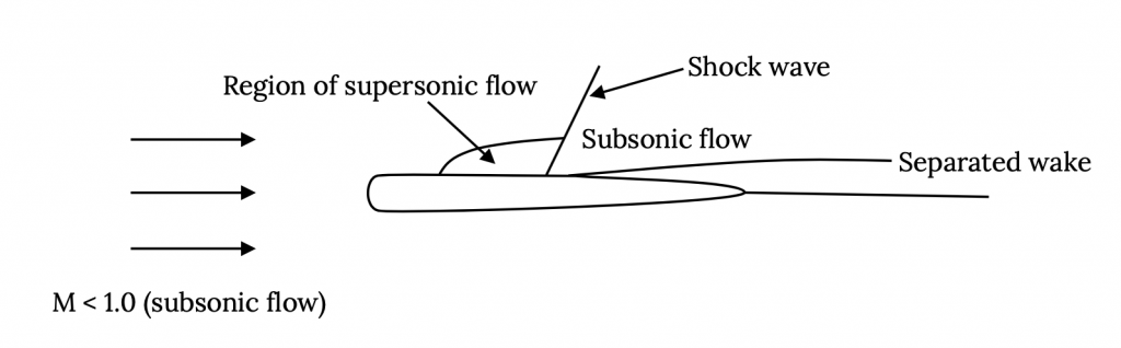
So at some high but subsonic speed (Mach number) supersonic flow over the wing has developed to the extent that a shock forms, and drag increases due to a separated wake and losses across the shock. The point where this begins to occur is called the critical Mach number, Mcrit. Mcrit will be different for each airfoil and wing shape. The result of all this is a drag coefficient behavior something like that shown in the plot below:
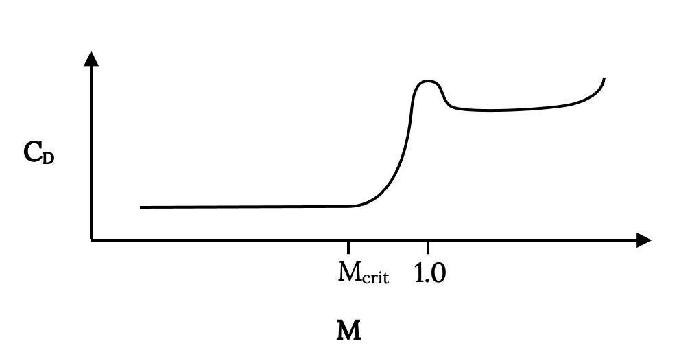
Actually the theory for subsonic, compressible flow says that the drag rise that begins at the critical Mach number climbs asymptotically at Mach 1; hence, the myth of the “sound barrier”. Unfortunately many people, particularly theoreticians, seemed to believe that reality had to fit their theory rather than the reverse, and thought that drag coefficient actually did become infinite at Mach 1. They had their beliefs reinforced when some high powered fighter aircraft in WWII had structural and other failures as they approached the speed of sound in dives. When the shock wave caused flow separation it changed the way lift and drag were produced by the wing, sometimes leading to structural failure on wings and tail surfaces that weren’t designed for those distributions of forces. This flow separation could also make control surfaces on the tail and wings useless or even cause them to “reverse” in their effectiveness. The pilot was left with an airplane which, if it stayed together structurally, often became impossible to control, leading to a crash. Sometimes, if the plane held together and the pilot could retain consciousness, the plane’s Mach number would decrease sufficiently as it reached lower altitude (the speed of sound is a function of temperature and is higher at lower altitude) and the problem would go away, allowing the pilot to live to tell the story.
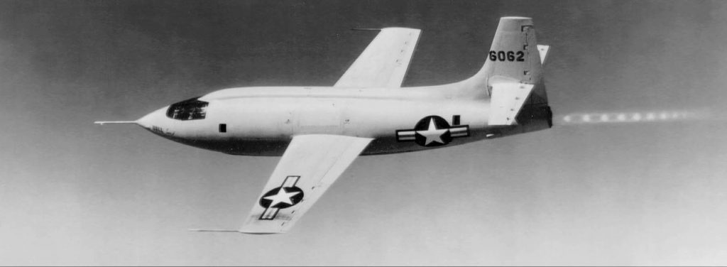
At any rate, experimentalists came to the rescue, noting that bullets had for years gone faster than the speed of sound (“you’ll never hear the shot that kills you”) and designing a bullet shaped airplane, the Bell X-1, with enough thrust to get it to and past Mach 1.
Once the plane is actually supersonic, there are actually two shocks on the wing, one at the leading edge where the flow decelerates suddenly from supersonic freestream speed to subsonic as it reaches the stagnation point, and one at the rear where the supersonic flow over the wing decelerates again. As a result, the “sonic boom” one hears from an airplane at supersonic speeds is really two successive booms instead of a single bang.
So it is important that we be aware of the Mach number of a flow because the forces like drag can change dramatically as Mach number changes. We certainly don’t want to try to predict the forces on a supersonic aircraft from test results at subsonic speeds or vice-versa. On the other hand, as long as everything we are considering happens below the critical Mach number we may not need to worry about these “compressibility effects”. In general, below Mcrit we can consider the flow to be “incompressible” and assume that density is a constant. Above Mcrit we can’t do this and we must use a compressible form of equations like Bernoulli’s equation.
Based on the above, one name we often give to the Mach number is a “similarity parameter”. Similarity parameters are things we must check in making sure our experimental measurements and calculations properly account for things such as the drag rise that starts at Mcrit. We don’t want to try to predict compressible flow effects using incompressible equations or test results or vice-versa.
The other three terms in our force relationship are also similarity parameters. Let’s look at the first term on the right hand side of that relationship. This grouping of terms is known as the Reynolds Number. Reynolds Number may be seen in different texts abbreviated in different ways [Re, Rn, R, Rex, etc.] depending on the convention in the field of use and on its application. Here we will use Re.

Reynolds number is really a ratio of the inertial forces and viscous forces in a fluid and is, in a very real way, a measure of the ability of a flow to follow a surface without separating.
Reynolds number is also an indicator of the behavior of a flow in a thin region next to a body in a flow where viscous forces are dominant, determining whether that flow is well behaved (laminar) or randomly messy (turbulent). This thin region is called the boundary layer.
Inertial forces are those forces that cause a body or a molecule in a flow to continue to move at constant speed and direction. Viscous forces are the result of collisions between molecules in a flow that force the flow, at least on a microscopic scale, to change direction. The combination of these forces, as reflected in the Reynolds Number, can lead a flow to be smooth and orderly and easily break away from a surface or to be random and turbulent and more likely to follow the curvature of a body. They also govern the magnitude of friction or viscous drag in between a body and a flow.
In general, a laminar boundary layer , which occurs at lower Reynolds Numbers, results in low friction drag (skin friction) but isn’t very good at resisting separation and may promote a large “wake” drag. A turbulent boundary layer , which occurs at higher Reynolds Numbers, has higher friction drag but resists flow separation better leading to lower “wake” drag. So which do we want? This all depends on the shape of the body and the relative magnitudes of wake and friction drag.
A classic case to examine is the flow around a circular cylinder or, in three dimensions, over a sphere.
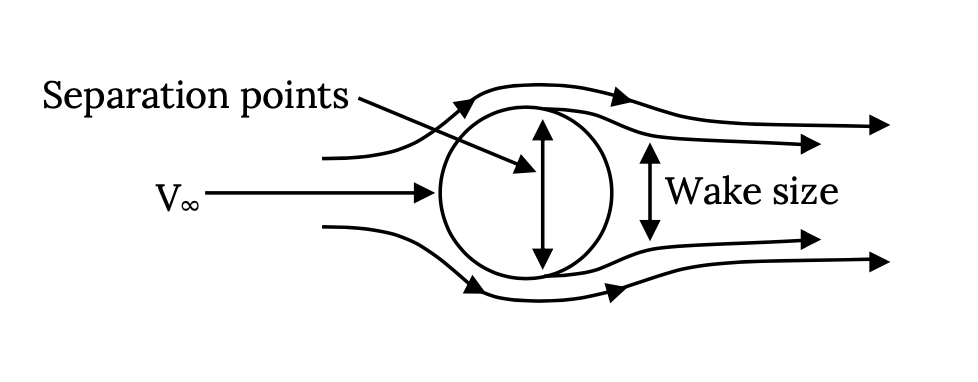
Flow over a circular cylinder or sphere will generally follow its surface about half way around the body and then break away or separate, leaving a “wake” of “dead” air. This wake causes a lot of drag. This wake is similar to that seen when driving in the rain behind cars and especially large trucks. On a truck the point where the flow separates is about at the rear corners of the trailer body or tailgate. On a car it is often less well defined with separation occurring somewhere between the top of the rear window and the rear of the vehicle. On an aerodynamically well designed car the separation point would be right at the rear deck corner or at the “spoiler” if the car has one. A small wake gives lower drag than a large wake.
On a circular cylinder or sphere the separation point will largely depend on the Reynolds Number of the flow. At lower values of Re the flow next to the body surface in the “boundary layer tends to be “laminar”, a flow that is not very good at resisting breaking away from the surface or separating. Lower Re will usually result in separation somewhat before the flow has reached the half-way point (90 degrees) around the shape, giving a large wake and high “wake drag”. At higher Re the flow in the boundary layer tends to be turbulent and is able to resist separation, resulting in separation at some point beyond the half-way point and a smaller wake and wake drag.
Because the wake drag is the predominant form of drag on a shape like a sphere or circular cylinder, far greater in magnitude than the friction drag, the point of flow separation is the dominant factor in determining the value of the body’s drag coefficient.
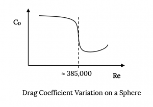
In the above graph the Reynolds Number is based on the diameter of the sphere and the drag coefficient drops from a value of about 1.2 to about 0.3 as the “critical” Reynolds Number is passed at a value of about 385,000. This is a huge decrease in drag coefficient and illustrates how powerful an influence Re can have on a flow and the resulting forces on a body.
Note that a flow around a cylinder or sphere could fall in the high drag portion of the above curve because of several things since Re depends on density, speed, a representative length, and viscosity. Density and viscosity are properties of the atmosphere which, in the Troposphere, both decrease with altitude. The major things affecting Re and the flow behavior at any given altitude will be the flow speed and the body’s “characteristic length” or dimension. Low flow speed and/or a small dimension will result in a low Re and consequently in high drag coefficient. A small wire (a circular cylinder) will have a much larger drag coefficient than a large cylinder at a given speed.
Of course drag coefficient isn’t drag. Drag also depends on the body projected area, air density, and the square of the speed:
")
Hence, it cannot be stated in general that a small sphere will have more drag than a large one because the drag will depend on speed squared and area as well as the value of the drag coefficient. On the other hand, many common spherically shaped objects will defy our intuition in their drag behavior because of this phenomenon. A bowling ball placed in a wind tunnel will exhibit a pronounced decrease in drag as the tunnel speed increases and a Reynolds Number around 385,000 is passed. A sphere the size of a golf ball or a baseball will be at a sub-critical Reynolds Number even at speeds well over 100 mph. This is the reason we cover golf balls with “dimples” and baseball pitchers like to scuff up baseballs before throwing them. Having a rough surface can make the boundary layer flow turbulent even at Reynolds numbers where the flow would normally be laminar.
The CD behavior shown in the plot above is for a smooth sphere or circular cylinder. The same shape with a rough surface will experience “transition” from high drag coefficient behavior to lower CD values at much lower Reynolds Numbers. A rough surface creates its own turbulence in the boundary layer which influences flow separation in much the same way as the “natural” turbulence that results from the forces in the flow that determine the value of Re. Early golfers, playing with smooth golf balls, probably found out that, once their ball had a few scuffs or cuts, it actually drove farther. They probably then started experimenting with groove patterns cut into the surface of the balls. This led to the dimple patterns we see today which effectively lower the drag of the golf ball (this is not all good since the same dimples make a golfer’s hook or slice worse). The stitches on a baseball have the same effect, and baseball pitchers have found in their own somewhat unscientific experiments that further scuffing the cover of a new ball can make it go faster just as spitting on it can make it do other strange things.
The sphere or cylinder, as mentioned earlier, is a classic shape where there are large Re effects on drag. Other shapes, particularly “streamlined” or low drag shapes like airfoils and wings, will not exhibit such dramatic drag dependencies on Re, but the effect is still there and needs to be considered.
Like Mach number, Re is considered a “similarity” parameter, meaning that it we want to know what is happening to things like lift and drag coefficient on a body we must know its Reynolds Number and know which side of any “critical Re” we might be on. Flow over a wing could be quite different at sub-critical values of Re than at higher values, primarily in terms of the location of flow separation, stall, and in the magnitude of the friction drag that depends on the extent of laminar and turbulent flow on the wing surface.
So in doing calculations and wind tunnel tests we need to look at the magnitude of Re and its consequences. In doing so, we can get into some real quandaries when we test scale models in a wind tunnel. If we, for example, test a one-tenth scale model of an airplane in a wind tunnel our “characteristic dimension” in the Reynolds Number will be 1/10 of full scale. So, if we want to match the test Re with that of the full scale plane, one of the other terms must be changed by a factor of ten. Changing velocity by an order of magnitude to ten times the full scale speed will obviously get us in trouble with the other similarity parameter, Mach number, so that won’t do any good. We must change something else or “cheat” by using artificial roughness to create a turbulent boundary layer when the value of Reynolds number is really too low for a turbulent boundary layer.
One of the biggest breakthroughs in aeronautics came in the 1920s when the National Advisory Committee for Aeronautics (the NACA) at Langley Field, VA built what they called a “Variable Density Wind Tunnel”. This was a test facility where the air density could be increased by a factor of 20, allowing the testing of 1/20 scale models at full scale Reynolds Numbers. The VDWT, now a National Historical Monument, was a subsonic wind tunnel built inside of a egg-shaped pressurized steel shell. Quite sophisticated for its time, the tunnel was pressurized to 20 atmospheres after the wing model was installed. The tunnel was operated and the test model was moved through a range of test angles of attack by operators who observed their tests through pressure tight windows that resembled ship portholes. The model wings, each with a five inch chord and a thirty inch span, were machined to very tight tolerances based on dimensions worked out by NACA scientists and engineers. For the first time the world of aeronautics had reliable, full scale aerodynamic measurements of wings with a wide range of airfoil shapes.
Today in wind tunnel testing we usually “cheat” on Reynolds Number by using “trip strips”, small sandpaper like lines placed near the leading edges of wings and fuselages to force the flow to transition from laminar to turbulent flow at locations calculated prior to the tests. Although the Variable Density Wind Tunnel was retired long ago, we still have a unique capability at what is now NASA-Langley Field with the National Transonic Facility, a wind tunnel in which the working gas is nitrogen at temperatures very near its point of liquification. Since density, viscosity, and speed of sound all change with temperature it is possible in the NTF to simulate full scale Reynolds Numbers and Mach numbers at the same time. While testing is not easy at these low temperatures, properly run investigations in the NTF can yield aerodynamic data that can be obtained in no other manner.
In concluding this discussion of Reynolds Number it should be noted that the “characteristic length” in Re may take several different values depending on convention and that the value of Re at which transition from laminar to turbulent flow occurs can also vary with application. As shown earlier, we base the Reynolds Number for a circular cylinder or sphere on its diameter. The transition Re is just under 400,000. However, if we were mechanical or civil engineers working with flows through pipes, we would use the pipe diameter as our dimension and we would find that transition takes place at Re of about 5000, some two orders of magnitude different from transition on the sphere. We need to be aware of this different perspective on the important magnitudes of Re when talking with our friends in other fields about flows.
When we are talking about the value of Reynolds Number on a wing or an airplane the characteristic dimension used is the mean or average chord of the wing, the average distance from the wing’s leading to trailing edge. When we are doing detailed calculations on the behavior of the flow in the boundary layer we will use yet another dimension, the distance from the stagnation point over the surface of the body to the point where we are doing the calculations.
OK, we have found our something about the importance of Mach Number and Reynolds Number, what about the other two groupings of parameters in the force dependency equation we had earlier?
There were two other terms, gl/V2, and P/ρV . The first of these is a ratio of gravitational and inertial forces and relates to forces which arise as a consequence of a body being close to an “interface” such as the ground or the surface of the ocean. This term is usually inverted and its square root is known as the Froude Number.
Froude Number = V / [gl]1/2 ,
where the length in the equation is the distance between the body and the fluid interface; i.e., the height of the airplane above the runway or the depth of a submarine below the surface. Unless that distance is less than about twice the diameter of the submarine or the chord of the wing, Froude Number can be generally ignored; but within this range, it can help account for increases in drag or lift that may occur when a body is near a surface.
The final term, the Euler Number, P/ρV, is really not important in air, but is used when looking for the likelyhood of cavitation effects on a body in water. When the pressure in water is lowered to the vapor point of water at a given temperature, the water will boil even though temperature is lower than its usual boiling point. When flow accelerates around a ship propeller or hull the pressure can become low enough locally to boil the water, and this boiling or cavitation can cause serious increases in drag, noise, loss of propeller thrust, and damage to the surface itself. The term used to examine this is a modification of the one found in our analysis, rewritten slightly to account for the importance of the vapor pressure.
=[P−Pv]/ρV2")
Note that the denominator is a familiar grouping of parameters, twice the dynamic pressure.
1.14 Airfoils and Their Aerodynamic Coefficients
At the beginning of this text we looked at the terminology that is used to define the shape of the airfoil, things like chord, camber, and thickness, as well as the things like span, chord, sweep, and aspect ratio which define the shape of a complete wing. In the section above we found that the best way to talk about the forces acting on an airfoil (2-D) or a wing (3-D) is in terms of non-dimensional coefficients. Let’s take a look again at those coefficients and how they are defined in both two and three dimensions and look at the way these change as a function of the wing or airfoil angle of attack to the flow.
A few pages back we defined the lift and drag coefficients for a wing. These are repeated below and are extended to define a pitching moment coefficient:
Note again that the area “S” is the “planform” area of the wing, the “projected” area one would see looking down on the wing and not its actual surface area. The moment coefficient has a slightly different denominator which includes the mean or average chord along with the planform area in order to make the coefficient unitless, since the pitching moment has units of force times distance. A little later we will look at the moment in more detail and see what reference point(s) should be used in measuring or calculating that moment.
The coefficients above are in three-dimensional form and are as we would define them for a full wing. If we are just looking at the airfoil section, a two-dimensional slice of the wing, the area in the denominator would simply become the chord.
It would be helpful to know something about the typical ranges of these coefficients in either two or three dimensions so we will have some idea how valid our calculations may be.
-2.0 < CL < +2.0 for a normal wing or airfoil with no flaps
-3.0 < CL < +3.0 for a wing or airfoil with flaps
0.005 < CD < 0.025 for a wing or airfoil (more for a whole airplane)
-0.1 < CM < 0.0 for a wing or airfoil when measured at c/4
It should also be noted that the pitching moment is defined as positive when it is “nose up”. Depending on the direction of the airfoil or wing within an axis system this may be counter to mathematical custom. In fact, most texts commonly treat aerodynamics problems as if the freestream velocity is coming from the left in the positive x direction and the wing or airfoil is facing toward the left in a negative x direction. In such a depiction a positive pitching moment would be clockwise even though customary mathematical treatment would assign this a negative sign.
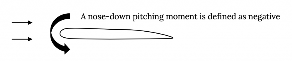
1.15 Angle of Attack
We also need to define the way we relate the orientation of the wing to the flow; i,e., the wing or airfoil angle of attack, α. At the same time we can look at the definition for the direction of lift and drag.
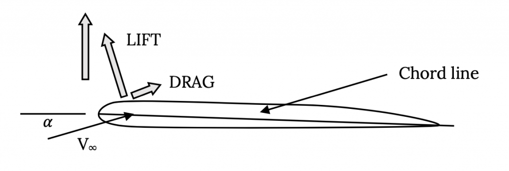
Note that the angle of attack, α, is defined as the angle between the wing or airfoil chord and the freestream velocity vector, not between the velocity and the horizontal. Also note that Lift and Drag are defined as perpendicular and parallel, respectively, to the freestream velocity vector, not “up and back” or perpendicular and parallel to the chord. These definitions often require care because they are not always intuitive. In many situations the force we define as lift will have a “forward” component to it along the wing chord line. This is, in fact, the reason that helicopter and gyrocopter rotor blades can rotate without power in what is known as the “autorotation” mode, giving lift with an unpowered rotor.
Given these definitions lets look at the way lift and drag coefficient typically change with angle of attack.
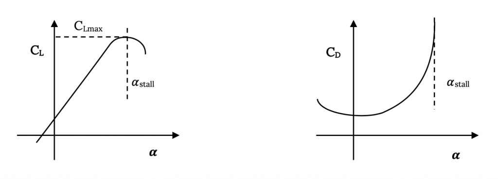
Let’s look at a few things in the above plots:
-
- The lift coefficient varies linearly with angle of attack until the wing approaches stall. Stall begins when the flow begins to break away or separate from the wing’s upper surface and may progress quickly or gradually over the surface.
- When the lift coefficient no longer increases with angle of attack, in the middle of stall progression, we have CLmax the largest value of lift coefficient we can get for a particular airfoil or wing at a given Reynolds number. The value of CLmax will, in general, increase with increasing Re.
- The lift coefficient is not shown as zero in value at a zero angle of attack. On a “symmetrical” airfoil; i.e., one with no camber, the lift will be zero at zero angle of attack. On a cambered airfoil the lift will be zero at some negative angle of attack which we call the “zero lift angle of attack”, αL0.
- Drag increases rapidly in stall.
We should explore this idea of stall further because something seems amiss here. The plot above shows that stall is where we have our maximum lift coefficient. How can that be true when we’ve always been told that stall is where an airplane looses lift?
Our dilemma here stems from the meanings of two different terms, lift and lift coefficient. Let’s look at the relationship between lift and lift coefficient.
Lift=CL[1/2ρV2S]
To have lift we must have two things, a good lift coefficient and the speed necessary to turn that lift coefficient into lift. So what is the problem here? The problem is drag.
When an airplane reaches CLmax it has its highest possible lifting capability or lift coefficient. But looking at the other plot, the one of drag coefficient, we see that it also has a rapidly increasing drag coefficient. The resulting drag causes a reduction in speed and, since speed is squared in the relationship above it has a much more powerful influence on lift than does the lift coefficient. Lift decreases as the speed drops and, indeed, even though we have a very high lift coefficient we can’t make enough lift to overcome the plane’s weight. And, as we can see from the plot on the left, if we go past the stall angle of attack we also get a decrease in lift coefficient.
As noted above up until stall the lift coefficient is shown to vary linearly with angle of attack and to become zero at the zero lift angle of attack L0. Given this we can write a simple equation for the value of CL.
Theory will show and experiment will verify that for an airfoil section (a two dimensional slice of a wing) this slope, dCL /dα, is equal to 2π, where the angles of attack are expressed in radians. So theoretically for an airfoil section this equation becomes:
![CL=2π[α−αL0]](https://eng.libretexts.org/@api/deki/files/49085/b32694dc3cfa9c46969bb541597b89a8.png?revision=1 "CL=2π[α−αL0]")
For a three dimensional wing the slope of the curve may be less and both theory and experiment can be used to determine that 3-D slope.
So how does the shape of the airfoil section influence this relationship? First, the shape of the camber line will determine the value of the zero lift angle of attack. We will find in a later course in aerodynamics that there are ways to calculate L0 from the shape of the airfoil camber line.
It is harder and may even be impossible to calculate the value of CLmax and the angle of attack for stall. These are functions of the thickness of the airfoil and the shape of its surface as well as of things like the Reynolds Number. We have to look at friction effects and Boundary Layer Theory to even begin to deal with the stall region successfully. Our only alternative is to use wind tunnel testing. And this is what the people at the National Advisory Committee for Aeronautics (NACA) which was mentioned earlier did in their Variable Density Wind Tunnel.
1.16 NACA Airfoils
In the 1920s the scientists and engineers at the NACA set out to for the first time systematically examine how things like camber line shape and thickness distributions influenced the behavior of airfoils. They began their quest by deciding how to define an airfoil shape using only three numbers and four digits. They looked at the best airfoil shapes of their time and found a good way to vary the thickness of the airfoil from its leading edge to the trailing edge and wrote an equation for this distribution that allowed everything to be defined in terms of one, two-digit number. Then they wrote two equations for the airfoil camber line, one for the front part of the wing up to the point of maximum camber and the other for the aft part of the wing behind the maximum camber location. These two equations depended on two single-digit numbers, one giving the location of the maximum camber point in tenths of the chord and the other giving the maximum distance between the camber and chord lines in hundredths of the chord. Then they used these four digits to identify the resulting airfoil.
For example, the NACA 2412 airfoil is an airfoil where each of the numbers means something about the shape:
2 – The maximum distance between the chord and camber lines is 2% of the chord.
4 – The location of the point of maximum camber is at 40% chord.
12 – The maximum thickness of the airfoil is 12% of the chord.
These four digits (three numbers) could then be used with related equations to draw the airfoil shape.
Using this method the NACA could systematically look at the effects of just the amount of maximum camber by testing a series of shapes such as 1412, 2412, 3412, etc. , or they could hold the maximum camber steady and look at the effect of placement of maximum camber (2212, 2312, 2412, 2512, etc.) , or fix the shape of the camber line and look at the effect of thickness variation (0006, 0009, 0012, 0015, 0021, etc.). Note that this last set of airfoils are all symmetrical; i.e., zero camber. And this is precisely what was done with tests on hundreds of airfoils. A wide variety of airfoils were tested in the Variable Density Wind Tunnel and the results plotted. Sample plots are presented in Appendix A.
The first set, Figures A-1 (A&B), is for an NACA 0012 airfoil section. Note that this is a symmetrical airfoil section (the first zero indicates that there is no camber and thus the second number is meaningless) and has a 12% thickness. We first see that there are several plots on each of the two graphs and that there are multiple definitions of the vertical axis for each plot. On the left hand plot the horizontal axis is the angle of attack given in degrees and the primary vertical axis is the section or two-dimensional lift coefficient. There is also a secondary vertical axis for the pitching moment coefficient (with the moment measured relative to c/4, the quarter chord ).
There is a lot of information given on plot A. The first thing we note is that there are two sets of lift coefficient curves and that each of these seems to have a couple of different plots of the stall region. Note that the linear portion of one set of these curves goes through the plot axis showing that the lift coefficient is zero at an angle of attack of zero. These curves are for the basic 0012 airfoil which is a symmetrical airfoil and will have no loft at zero angle of attack.
There are, as noted above, at least two different stall region plots for this symmetrical airfoil. To understand these we need to look at the inset information about Reynolds number (noted as simply “R” on these plots). There are four different symbols shown in this inset. The “diamond” symbol denoted data for the wing tested at a Reynolds number of 9 x 10⁶, the square for Re = 6 x 10⁶, and the circle for Re = 3 x 10⁶. The other symbol, a triangle, is for the airfoil tested with a “standard roughness” or a roughened surface at a Re = 6 x 10⁶. Usually the higher the value of Reynolds number the higher the value of maximum lift coefficient but in this particular case there is only a slight increase with CLmax moving up from about 1.5 to 1.6 as Reynolds number on the smooth airfoil increases from 3 to 6 x 10⁶. For the smooth surface stall always occurs at 16 degrees angle of attack. Note also that the airfoil also stalls at minus 16 degrees angle of attack, verifying its symmetrical behavior. The rough surface causes a much earlier stall and lower value of CLmax.
So, what is the other set of “lift curves” that are displaced up and to the left on this plot? These are the data for the 0012 airfoil with a trailing edge flap. Other inset information on the plot tells us that this is a split flap with a chord of 20% of the airfoil chord and it is deflected 60 degrees. Note that the basic airfoil is drawn to scale on the right hand plot and the flap and its deflection are noted in dashed lines on the drawing.
This data shows that for this particular flap the lift curve shifts to the left such that it has zero lift at minus 12 degrees, in other words αLO, the zero lift angle of attack, is minus 12 degrees for the flapped airfoil. The curves show that the deflection of the flap has increased CLmax from about 1.6 up to about 2.4, a 50% increase. CLmax for the rough surface airfoil has gone from 1.0 to 1.9.
Now, there are two other curves on this plot. They are curves for the pitching moment coefficient about the quarter chord, with and without flap deflection. First note that the scale to the left of the plot is different for moment coefficient than it was for lift coefficient. Do not confuse these two scales. Next, note that the upper of these two curves is for the wing without flaps and that it has a value of zero over the range of angle of attack where the lift curve is linear. This means that the pitching moment is zero at the quarter chord for this airfoil. This is true for all symmetrical airfoils. We define the place where the pitching moment is zero as the center of pressure (sometimes called the center of lift) and we define the place where the pitching moment coefficient is constant with changing angle of attack as the aerodynamic center. We will look at these further a little later. For a symmetrical airfoil the center of pressure and the aerodynamic center are both at c/4.
Now let’s look at the plot B for the 0012 airfoil. This plot displays test results for drag coefficient and moment coefficient and plots them versus the lift coefficient, not the angle of attack. So to find the drag coefficient at a certain angle of attack requires us to first find the value of CL at that angle of attack and then use it to find CD.
Again on this plot there are different sets of data for different values of Reynolds number and roughness. Note that CD is smallest at zero angle of attack for this symmetrical airfoil as would be expected, and that as angle of attack is increased CD increases. The moment curve on this plot is for the moment coefficient at the aerodynamic center and not for c/4 as in the plot on the left. However, as noted above, for a symmetrical airfoil the aerodynamic center is at the quarter chord so these are the same here.
The next plot in Appendix A, Figure A-2 (A&B), shows similar data for the NACA 2412 airfoil. Like the 0012 airfoil this shape has 12% thickness but now it has a slight (one percent) camber with the maximum camber located at 40% of the chord. So we can compare these plots with the first ones to see the effect of added camber. Looking at all the same things mentioned above we see that the airfoil now has a positive lift coefficient (0.15) at zero angle of attack and that the zero lift angle of attack is now minus-one degree. CLmax is still about 1.6 for the unflapped wing but with flap deflection it has increased slightly from the symmetrical case. Pitching moment coefficient is no longer zero at c/4 but it is still constant, now at a value of about – 0.025 ; i.e., a slightly nose down pitching moment. Since the pitching moment at c/4 is still constant this point is still the aerodynamic center but it is no longer the center of pressure. The minimum drag coefficient is about the same as for the symmetrical wing and it is still minimum at about zero angle of attack but this is no longer at zero lift coefficient.
We can see the result of further increases in camber to two percent in the plots for the NACA 2412 airfoil. There is no data for flap deflection included in these plots. In this plot we can see that the pitching moment continues to increase negatively (nose down) as camber is increased and that the minimum drag coefficient has also begun to increase. The zero lift angle of attack and the lift at zero angle of attack are both seen to continue to increase in magnitude as camber is added as theory would suggest.
The next plots, Figure A-3 (A&B), for the NACA 2415 show very slight changes in the airfoil behavior with increased thickness from 12% to 15% but for the NACA 2421 section we see that the added thickness is resulting in earlier stall, decreased CLmax, increased drag coefficient, and in a non-linear moment coefficient variation with angle of attack about the quarter chord. This might suggest to us that 21% thickness is a little too thick.
The data (Figure A-4 (A&B), for the NACA 4412 airfoil continues to illustrate the trends discussed above, looking at the effect of adding more camber.
The last two plot sets, Figures A-5 and A-6, are for a different design of airfoil, the NACA 6-series airfoil, a shape we will discuss first before looking further at the graphs.
The NACA tested a wide variety of airfoil shapes in its four digit series investigations. However there were some limits to the shape variations one could get using the four digit designation. They couldn’t, for example, look at an airfoil with maximum camber at 25% of the chord, only 20% or 30%. Hence they went on to develop a 5 digit airfoil series. Later they looked at an airfoil series designed to optimize the use of laminar and turbulent flow in the boundary layer to minimize drag and developed the 6-series airfoils. Let’s look at both of these.
The NACA 5-digit series used the same thickness distribution as the four digit series but allowed more flexibility in defining the position of maximum camber. It also attempted to relate the amount of camber and the first digit in the airfoil designation to a “design CL”. The design CL is the lift coefficient viewed as optimum for the performance objectives of a given airplane. A long range transport may have a design lift coefficient of around 0.3 while a fighter aircraft might have a higher design CL. An example of an NACA 5-digit airfoil is given below with an explanation of the numbering system:
NACA 23021
2 – the maximum camber is approximately 0.02 and the design CL is 2 x 0.15 = 3.0
30 – the position of the maximum camber is (0.30/2) times the chord or 0.15c
21 – the maximum thickness is 0.21c
The NACA 6-series (note that this is simply called the “six” series and not the six digit series although most of the designation numbers do have six digits) was developed in the 1930s in an attempt to design a series of airfoil shapes which optimized the areas of laminar and turbulent flow in the boundary layer on the wing. As we discussed earlier, laminar flow in the boundary layer is a low friction flow and that is good; however, laminar flow is poor at resisting flow separation and separation results in high drag and low lift. A turbulent boundary layer is much better at resisting flow separation than a laminar one but it has higher friction drag.
Flow separation is much more likely when the flow is decelerating (where the pressure is increasing, known as an “adverse” pressure gradient because separation is likely). The flow over an airfoil will usually be accelerating over the front of the shape up to the point of its minimum pressure which us usually at about the point of maximum thickness. Here it is safe to have laminar flow because the flow is not likely to try to separate. If we want more laminar flow and, hence, a larger part of the airfoil with low friction drag, we can move the maximum thickness point more toward the rear of the airfoil. The idea is to get as large as possible an area of laminar flow and then let the boundary layer transition to turbulent flow before the thickness starts to decrease so the turbulent boundary layer will resist separation. This results in an airfoil with a smaller leading edge radius than the older designs and with the maximum thickness further back.
Two such 6-series shapes are sketched as part of their NACA data plots in Appendix A, the NACA 651-212 and 651-412 airfoils. One thing that is immediately obvious when comparing these two data plots to those of the NACA 4-digit airfoil data is the “bucket” in the center of the drag coefficient curves in the right hand plots. This so-called “drag bucket” is characteristic of the 6-series airfoils. All of these airfoils have a region of angle of attack or lift coefficient over which the drag is considerably lower than at other angles of attack. This is the range of angle of attack where laminar flow can exist over a large part the forward portion of the airfoil, giving a reduction in friction drag.
The 6-series airfoil numbering system is devised to help the designer/aerodynamicist select the best airfoil for the job by telling where the center of the “drag bucket” is located and telling the extent (width) of that drag bucket. In other words, if a designer wants a wing with an airfoil section that gives a design lift coefficient of 0.2 he or she wants the center of the drag bucket to be at a CL of 0.2 so the airplane will be able to do its design mission at the lowest possible drag conditions. Hence, one of the numbers in the 6-series designation tells the CL for the center of the drag bucket. Lets look at one of these airfoil designations and see what the numbers mean.
NACA 651-212
6 – this is merely the “series” designation
5 – the minimum pressure location at zero lift is at 50% chord
1 – this is a subscript which may or may not appear in a 6 series designation. It means that the width of the “drag bucket” extends for a range of CL of 0.1 above and below the design CL
2 – the design CL is 0.2
12 – as always, the maximum thickness as a % chord
Now if we again look at the data for the above airfoil we see that the drag bucket is indeed centered at a lift coefficient of about 0.2 and the bucket extends for at least a CL range of 0.1 on both sides of its center. Similarly if we look at the plots for the NACA 651-412 we find that the drag bucket is further to the right and centered at about a CL of 0.4.
A closer comparison of these 6-series aerodynamic data with those of the 4-digit series cases will show that not everything is better. The 6-series airfoils often stall a little earlier due to their smaller leading edge radii and hence have slightly lower CLmax values than their earlier counterparts. Also their drag coefficients outside of the range of the drag bucket may be higher than conventional airfoils. As in all things in real life improvements in one area are often accompanied by penalties in others. Nonetheless, the 6-series airfoils are excellent designs and are still used today on many aircraft.
1.17 Pitching Moment
Before we look further at airfoil development we should step back a bit and look further at two things mentioned earlier, the aerodynamic center and the center of pressure. These are two important points on the airfoil that depend on the behavior of the pitching moment. A moment must be referenced to a point and these happen to be very meaningful points about which to reference the pitching moment on an airfoil or wing.
The moment on an airfoil is related primarily to the way lift is produced on the shape. Drag also contributes to the moment but to a much smaller extent. At subsonic speeds the lift on most airfoils is higher on the front part of the shape than at the rear and might look something like this:
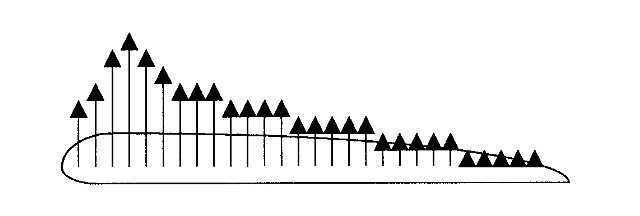
If we choose to talk about the pitching moment about the airfoil leading edge, the moment would always be nose down or counterclockwise. If we sum up the moments at some point about half way back along the chord the moment would be nose up or clockwise since the lift forces to the left are greater than those on the right. Obviously there is some point between the airfoil leading edge and its center where the moments would sum to zero. This would be the center of pressure. It might be interesting and useful to know where this place is since it seems to be a natural balance point or sorts. The only problem is that this position may move as the airfoil changes angle of attack. For example, at higher angle of attack even more of the lift might be produced near the front of the airfoil and the center of pressure would move closer to the nose of the airfoil.
As it turns out, according to aerodynamic theory which you will examine in a later course, there is another point which is of even more interest, the aerodynamic center. This is the point where the moment coefficient (not the moment itself) is constant over a wide range of angle of attack. Basic aerodynamic theory will tell us that this is approximately at the quarter-chord of the airfoil in subsonic flow. This was seen to be the case for the airfoils whose data are shown in Appendix A.
Theory will also show and experiment will verify that for a symmetrical airfoil such as the NACA 0012 shape in Appendix A the aerodynamic center and the center of pressure are in the same place. In other words, for symmetrical airfoils at the aerodynamic center the pitching moment is not only constant but is also zero. This makes the aerodynamic center a very convenient place to locate major structural elements or to use as the balance point for control surfaces.
1.18 Camber and Flaps, and Flight at Reduced Speeds
We have seen in the data of Appendix A that as the camber of a wing increases its aerodynamic performance changes. Looking at the data for the NACA 0012, 1412, and 2412 airfoils we saw that as camber (indicated by the first term in the NACA four digit numbering system) is increased the lift curve shifts to the left giving more lift coefficient at zero angle of attack, an increasingly negative angle of attack for zero lift coefficient, and a slowly increasing value of maximum lift coefficient. This is accompanied by a slight increase in drag coefficient and a negative increase in pitching moment coefficient at the aerodynamic center as camber increases. In later aerodynamics courses you will learn how to predict these changes which result from modification of the airfoil camber line shape. It is evident now, however, that increasing camber can give higher lift coefficients and both the airplane designer and the pilot may wish to take advantage of this. One type of flight where this becomes very useful is low speed flight, especially in takeoff and landing.
To fly the lift of the airplane must equal its weight.
ρV2S")
This relationship says that lift comes from four things, the lift coefficient, the density, the velocity, and the wing planform area. There is nothing much we can do about the density, it comes with the altitude, and while there are ways to change the wing area while a plane is in flight, these are often impractical. We note that speed is a powerful factor since it is squared.
The equation above essentially tells us that if we want to fly at a lower speed with a given wing and altitude we must increase the lift coefficient. We can do this to a certain extent as we increase the angle of attack from the zero lift angle of attack to the angle for stall, but stall defines our limit.
ρVstall2S")
We, of course, don’t want to try to fly at CLmax because we will stall, but the stall speed does define the minimum limit for our possible range of flight speed at a given altitude. If we want to fly at lower speed we need to increase the value of CLmax. The graphs in Appendix A show us that this can be done with flaps. On the plot for the NACA 1412 airfoil we see that by deflecting a split flap with a length of 20% of the airfoil chord to an angle of 60 degrees we can increase the maximum lift coefficient from 1.6 to 2.5, a change which would lower our stall speed by 20 percent. This means that we can fly at a 20% lower speed.
This is a powerful effect but it isn’t free. It is accompanied by a large increase in drag coefficient and a huge change in pitching moment. This may mean a need for a larger horizontal stabilizer or canard to counter the pitch change and we will need to deal with the drag.
In the early days of flight there was no real need for flaps. Aircraft flew at speeds very slow by today’s standards and their stall speeds were often very low due to large wing areas. But as research showed how to reduce airplane drag and better engines gave increasingly more power and thrust not as much wing area was needed to cruise at the resulting higher speeds. Airplane designers found that making a plane cruise at over 200 mph and still land at something like 60 mph or less was a problem. Landing speed is important because it is directly related to stopping distance and the needed runway length. Higher landing speeds also may increase the risk of landing accidents.
Most airplanes cruise at a lift coefficient of about 0.2 to 0.3 and the best subsonic airfoils will have a CLmax no higher than 1.8. These two factors define the problem of high speed cruise and low speed landing.
In 1933 the Boeing Company brought out the Boeing 247 airliner, a thoroughly modern plane for its time which took advantages of all the accumulated progress in engine and airframe design. Its cruise speed was 188 mph at an altitude of 8000 feet. The 247 weighed 13,650 pounds and had a wing area of 836 ft2. A quick calculation of its cruise lift coefficient gives CL = 0.23, a reasonable value. At that time existing runways required a landing speed of around 60 mph and a calculation of the 247’s lift coefficient at sea level at 60 mph gives 1.77, pretty near the maximum for a conventional wing.
The Douglas Aircraft Company (now a part of Boeing) decided to build a bigger and more comfortable airliner and came out with the DC-1, the prototype airplane, and the production model DC-2. The DC-2 weighed 36% more than the 247 at 18,560 pounds and had a slightly higher wing area of 939 ft2, but it cruised at about the same speed and altitude as its competitor. The cruise CL for the DC-2 comes out to be about 0.27, higher than the 247 because of its significantly larger weight. This higher “wing loading” gave the DC-2 passengers a more comfortable ride than the 247.
To land the DC-2 at 60 mph requires a CL of about 2.15, too high for a normal wing. The solution was to add flaps, giving extra camber and a higher CLmax when needed for landing and takeoff. This allowed the larger, more comfortable DC-2 to fly as fast as the 247 and still land and takeoff at all the commercial airports of its day. The DC-2 and its even larger and more comfortable sibling, the DC-3, went on to revolutionize the airline industry.
It should be noted that large flap deflections are used in landing where the added drag may actually be advantageous and smaller deflections are used in takeoff where lower drag and rapid acceleration are a must.
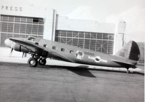

There are many types of flaps. There are both leading edge and trailing edge flaps and an array of variations on both. Aerodynamic theory tells us that a camber increase is most effective when it is made near the trailing edge of an airfoil, hence, the trailing edge flap is the primary type of flap used on wings. The deflection of virtually any type of trailing edge flap from a simple flat plate to a complex, multi-element flap system will shift the “lift curve” to the left and increase CLmax. Some trailing edge flaps have slots and multiple elements to help control the flow over the flaps and prevent separation to give even higher lift coefficient and often these flaps deploy in such a way as to temporarily add extra wing area.
Leading edge flaps do little to move the lift curve to the left but can do a lot to allow the airfoil to go to a higher angle of attack before stalling, by controlling the flow over the “nose” of the airfoil and delaying separation. Leading edge flaps are often used in takeoff and landing in conjunction with trailing edge flaps. A few aircraft have been designed with leading edge flaps or slots fixed permanently into the wing to give them lower stall speeds.
The effects of both leading and trailing edge flaps are shown in the following figure.
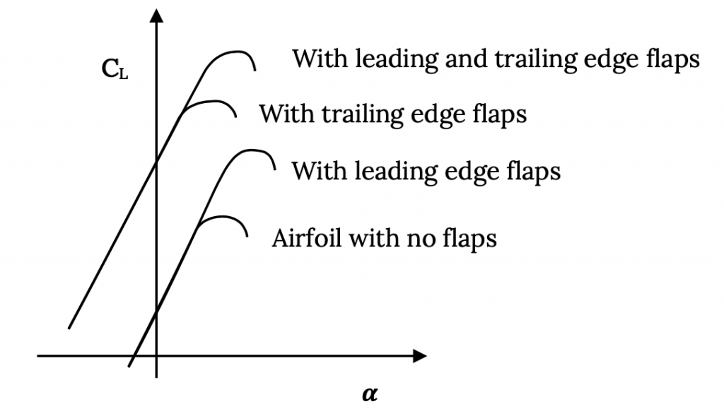
The following table lists typical magnitudes of lift coefficient with and with out both leading and trailing edge flaps for a “Clark Y” airfoil. The Clark Y airfoil is a famous non-NACA airfoil shape developed by Virginius Clark. Clark had served on the same commission as many of the founders of the NACA, a commission charged with studying European airfoil sections after World War I and, using much of the same information that the NACA used to develop its original 4 digit airfoils, Clark developed the Clark Y and other airfoils as part of his Ph.D research at MIT. In the Clark Y, Virginius Clark designed an airfoil shape with a flat bottom that made it easy to manufacture, and because of this and its excellent aerodynamic performance, it was used widely for everything from airplane wings to propeller blades.
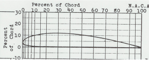
Table 1.3: Leading edge and trailing edge flap and slot effects on a Clark Y airfoil
| Configuration | C sub Lmax | alpha sub stall |
|---|---|---|
| Basic Clark Y airfoil | 1.29 | 15 |
| with 30% plain flap at 45° | 1.95 | 12 |
| with "fixed" slot and no flap | 1.77 | 24 |
| with slot and plain flap | 2.18 | 19 |
| with 40% Fowler flap at 40° | 3.09 | 14 |
| with deployable slot and Fowler flap | 3.36 | 16 |
To summarize, a trailing edge flap can have a significant “camber effect”; i.e., can shift the “lift curve” to the left, increasing the zero lift angle of attack and the value of CLmax. It can also be deployed in such a way as to temporarily increase wing area. A leading edge flap or slot will probably not produce a “camber effect” (if it does it is likely to be a “negative” one, slightly shifting the “lift curve” to the right) but will help retard stall to a higher angle of attack whether used on a wing with or without flaps.
1.19 Transonic and Supersonic Airfoils and Wings
Earlier we looked at the way flow can accelerate to supersonic speeds over an airfoil or wing as the free stream speed approaches the speed of sound and how, at Mach numbers higher than some “critical Mach number” the deceleration of that supersonic flow back to subsonic speeds can result in sudden flow separation and a drag increase. There are two ways to reduce this drag. One is by sweeping the wing and the other is by designing a special airfoil section.
1.20 Wing Sweep
The first way found to successfully decrease the drag rise that occurs in the transonic flight regime is by sweeping the wing. Theory and experiment showed that both the onset and the magnitude of the drag increase were functions of the “normal component” of the free stream Mach number, M∞. In other words, if a wing is swept 450 the normal component of the free stream Mach number is M∞ cosine θ or 0.707
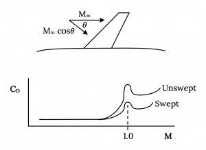
As with almost everything this benefit of sweep comes at a cost. Sweeping the wing also reduces its lift coefficient at a given angle of attack (reduces the slope of the lift curve) and the curved flow over the wing itself can lead to premature stall near the wing tips and a phenomenon known as “pitch up”
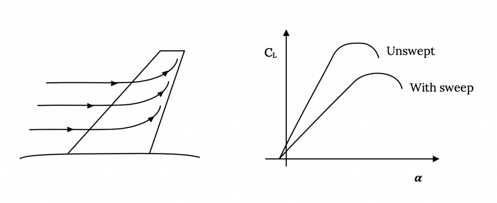
While most swept wings are angled toward the rear of the plane or swept back, theoretically it doesn’t matter whether the wing is swept forward or aft. Several early swept wing designs were drawn with forward swept wings which allowed the wing spar or structure to pass through the fuselage aft of the cockpit and presented fewer internal design problems but it was soon discovered that there was indeed a problem with forward swept wings. This problem was caused by the same type of curving flow that caused tip stall on the aft swept wings except that the result on the forward swept wing was an added lift at the wing tips that tended to twist the wings to their breaking point at fairly low speeds. There was little point in sweeping a wing to lower the transonic drag rise when the wing would break off long before such speeds were reached and the added weight needed to stiffen the wing to prevent failure made the airplanes too heavy. This problem was finally solved in the 1970s with the use of fabric based composite structures which could be designed in such a way that the wing got stronger as it tried to twist off. The X-29 experimental aircraft successfully proved that swept forward wings could indeed be used in transonic flows.
1.21 Supercritical Airfoils
The other method used to reduce the transonic drag rise on a wing was developed by Richard Whitcomb at NASA-Langley Research Center in the 1960’s. Dr. Whitcomb essentially reshaped the conventional airfoil section to do three things. He increased the “roundness” of the airfoil leading edge to give a more gradual acceleration of the flow to a speed lower than conventional airfoil shapes so when supersonic flow resulted on the surface it was weaker. He reduced the wing camber at its mid chord area to flatten the upper surface and allow a longer region of this weaker supersonic flow before allowing it to decelerate, giving less separation and drag. Finally, to make up for the lift that was lost by designing for slower upper surface flow, Whitcomb designed his airfoil with significant “aft camber” on its lower surface, noting that camber has a very powerful effect neat an airfoil trailing edge. The result was an airfoil somewhat like the one below which gave excellent aerodynamic performance with a reduced transonic drag rise. This type of airfoil is called a Whitcomb airfoil or a “supercritical” airfoil.
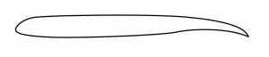
As it turned out, this airfoil was an excellent design for all ranges of flight with its only drawback being a tendency toward a large pitching moment due to the aft lower camber. Subsequent designs have reduced this problem and variants of this design are used on almost every type of aircraft today.
While discussing Richard Whitcomb and transonic flow, his “coke bottle” fuselage design should also be mentioned. In the early 1950’s as jet fighters were approaching Mach 1 in capability, the transonic drag rise of the whole airplane continued to be a problem in “breaking the so-called sound barrier”. Convair and the Air Force hoped that a new, highly swept, delta wing fighter designated the F-102 would be able to routinely fly at supersonic speeds; however two prototype aircraft failed to reach Mach 1. Whitcomb realized that, at the speed of sound, the air cannot be compressed any further and needs some place to go or it will simply push outward from the plane, displacing other airflow and causing drag. He suggested a redesign of the F-102 fuselage with a reduced cross section in the vicinity of the wing to allow this supersonic air a place to go without pushing away outer flows. The “wasp-waist” or “coke-bottle” fuselage was the result and the design which could formerly not make it to the speed of sound reached Mach 1.22 on its first flight.
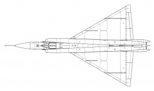
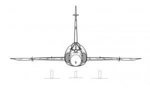
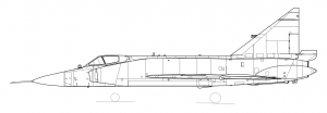
1.22 Three Dimensional Aerodynamics
Most of the things discussed in the previous sections were two dimensional phenomenon such as airfoil section design, the effects of camber, etc. Wing sweep was the exception. But there are many other variations in wing planform and shape that will influence the aerodynamic performance of a wing. Let’s start by looking at the Aspect Ratio.
A wing which is producing lift must have a lower pressure on its upper surface than on the lower surface. At the wing tips there is nothing to prevent the air from the lower surface from trying to go around the wing tip to the upper surface where the lower pressure acts like a vacuum. The result is some loss of lift near the wing tip. An ideal wing would have the same lift from wing tip to wing tip but a real wing doesn’t.
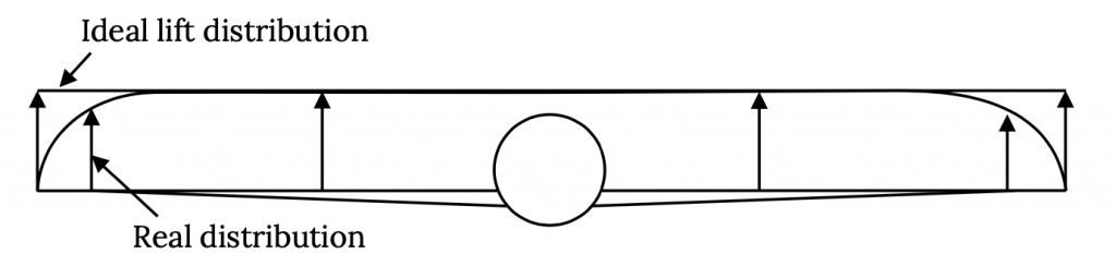
This loss of lift is felt for some distance inboard of the wing tips. The question is what percentage of the wing area this affects and this will depend on the wing Aspect Ratio, AR.
Aspect Ratio is a measure of the wing’s span divided by its “mean” or average chord. It can also be expressed in terms of the square of the span and the planform area.
AR = b2/S = b/cavg
where b = wing span, S = planform area, c = chord
To see why aspect ratio is important we can look at two different wing planforms of the same area but different aspect ratios.
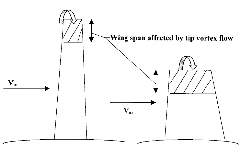
This flow around the wing tip results in two other problems, the production of a drag called the induced drag and the creation of a tornado-like swirling flow, called a wing-tip vortex behind the wing tip that can be a hazard to following aircraft.
The trailing vortices (one vortex from each wing tip) can continue for miles behind an aircraft and the “strength” of the vortices will depend on the weight of the generating aircraft. A following airplane, particularly a small one, may find itself suddenly turned upside down (or worse) if it encounters one of these vortices. This is particularly dangerous near the ground and is one of the reasons for required separation times between landing and taking off airplanes at airports.
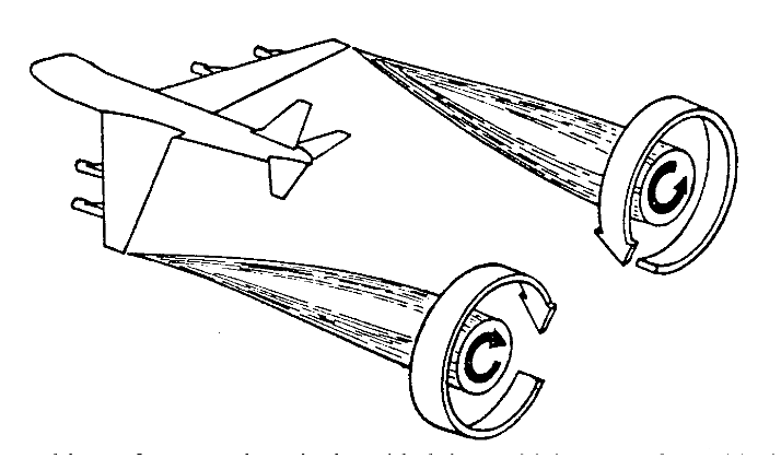
The 3-D problem of concern here is the added drag which comes from this flow around the wing tips and the decreased lift. Because of this flow the lift coefficient on a 3-D wing will be lower at a given angle of attack than a 2-D airfoil section of the same shape. Aerodynamic theory can be used to calculate the 3-D effect as a function of the planform shape of the wing and that effect can be characterized as an aspect ratio effect. A 2-D airfoil section is said to have an infinite aspect ratio and for the 2-D case theory gives a slope for the “lift curve” (dCL/dα) of 2π. For the 3-D case where aspect ratio is finite the slope of the lift curve will be found to decrease with decreasing aspect ratio.
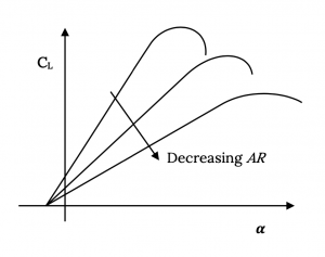
The added drag in 3-D comes from the same phenomenon that causes lift. We define life as a force perpendicular to the free stream velocity. Induced drag is a force that is perpendicular to the “downwash” velocity caused by the flow around the wingtip. This downwash velocity is small compared to the freestream flow and the induced drag is correspondingly small but it is still a force we need to understand and deal with.
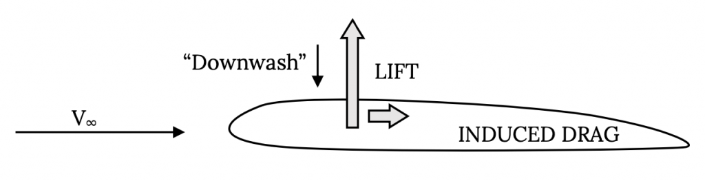
Theory will show the induced drag coefficient CDi to be:

From this it can be seen that as AR increases the induced drag decreases and that in the 2-D case where the theoretical aspect ratio is infinity, the induced drag coefficient is zero. But, what about the other term in the equation, e?
e is called the “Oswald efficiency factor”. The value of e will be somewhere between zero and one with one being the best or “minimum induced drag” case. Theory will show that e is a function of the way lift acts along the span of the wing which is a function of several things, including wing planform shape, wing sweep, wing twist, taper, the various airfoil sections used across the span, etc. A study of this theory will show that the best case, when e = 1.0 occurs when the lift is distributed along the wing span in an elliptical manner. This minimum induced drag case is often called the elliptical lift distribution case.
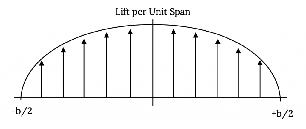
There are many ways to get an elliptical lift distribution. The easiest to visualize is that where the wing planform is shaped like an ellipse, that is where the wing chord varies elliptically along its span. In the 1940’s many World War II fighters were built with elliptical planforms to try to minimize induced drag. The most famous of these was the British Spitfire aircraft.
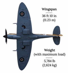
It is possible to get an elliptical or near-elliptical lift distribution in other ways with the right combination of wing taper, twist, and sweep or by varying the airfoil section used as you go out the span. Some of these combinations can give values of induced drag coefficient at or near a minimum while minimizing the difficulty of building the wing. In some cases a complicated planform is required for other reasons such as “stealth” or minimizing the radar return of the aircraft. The B-2, “stealth” bomber, despite its “saw-tooth” shaped wing planform, has a nearly elliptical lift distribution.
Often twist is part of this scheme because it may also be needed for control in stall. Because the control surfaces used for roll control, the ailerons, are near the wing tips we want to design the wing so the outboard portion of the wing will not stall when the inboard section begins to stall. For this reason the part of the wing near the tip is often twisted to give it a smaller angle of attack than the rest of the wing. Some airplanes use different airfoil sections near the tip than on the rest of the wing for this reason.
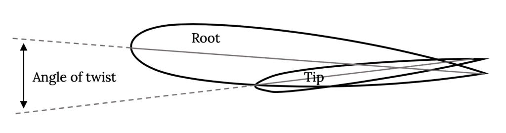
It should be stressed that while the elliptical lift distribution is ideal aerodynamically there are other factors which must be considered when designing the wing. For example, another lift distribution may well be the optimum one for structural strength or for control responsiveness. The British Spitfire was a very efficient airplane aerodynamically because of its elliptical wing planform but pilots found that they could not roll the fighter as quickly as their German opponents in dogfights. As a result the beautiful Spitfire wing was “clipped” in later versions to allow greater roll rates because in the real world of aerial warfare maneuverability was found to be more important than aerodynamic efficiency and drag.
It should also be stressed that induced drag is only a portion of the drag. This “drag due to lift” is independent of other sources of drag such as friction between the air and the “skin” or surface of the aircraft or the “pressure drag” which comes from the normal variation of pressures around the airfoil. These other types of drag must be calculated from aerodynamic theory and “boundary layer” theory, the subjects of two courses later in the curriculum.
Homework 1
1. Write a calculator or computer program to find standard atmosphere conditions (pressure, temperature and density) for any altitude in the troposphere and stratosphere in both SI and English units. Turn in a listing of the program and a print-out for conditions every 1,000 meters (SI units) and every 1000 feet (English units) up to 100,000 feet or 30,000 meters.
2. A compressed air tank is fitted with a window of 150 mm diameter. A U-tube manometer using mercury as its operating fluid is connected between the tank and the atmosphere and reads 1.80 meters. What is the total load acting on the bolts securing the window? The relative density of mercury is 13.6.
3. On a certain day the sea level pressure and temperature are 101,500 N/m2 and 25°C, respectively. The temperature is found to fall linearly with altitude to -55°C at 11,300 meters and be constant above that altitude.
4. An aircraft with no instrument errors and with an altimeter calibrated to ISA specifications has an altimeter reading of 5000 meters. What is the actual altitude of the aircraft? What altitude would the altimeter show when the plane lands at sea level?
References
Tables 1.1 and 1.2: National Advisory Committee for Aeronautics (1953). NACA-TR-1135 and NACA TN 1428. Retrieved from https://ntrs.nasa.gov/citations/19930091059
Figure 1.1: Kindred Grey (2021). “Airfoil Terminology.” CC BY 4.0. Adapted from James F. Marchman (2004). CC BY 4.0. Available from https://archive.org/details/1.1_20210804
Figure 1.2: Kindred Grey (2021). “Wing Planform Terminology.” CC BY 4.0. Adapted from James F. Marchman (2004). CC BY 4.0. Available from https://archive.org/details/1.2_20210804
Figure 1.3: Kindred Grey (2021). “Some Wing Planform Shapes.” CC BY 4.0. Adapted from James F. Marchman (2004). CC BY 4.0. Available from https://archive.org/details/1.3_20210804
Figure 1.4: Kindred Grey (2021). “A Typical Mechanical Sensitive Altimeter.” CC BY-SA 3.0. Adapted from WikiDot (2009). “Figure 4: The Mechanism.” CC BY-SA 3.0. Original: http://aviationknowledge.wikidot.com/aviation:sensitive-altimeters. Adapted: https://archive.org/details/1.4_20210804
Figure 1.5: James F. Marchman (2004). “Bernoulli’s Equation Example.” CC BY 4.0.
Figure 1.6: James F. Marchman (2004). “A Pitot Tube Measures Total Pressure.” CC BY 4.0.
Figure 1.7: James F. Marchman (2004). “A Static Tube Measures Static Pressure.” CC BY 4.0.
Figure 1.8: Kindred Grey (2021). “A Pilot-Static Probe.” CC BY 4.0. Adapted from James F. Marchman (2004). CC BY 4.0. Available from https://archive.org/details/1.8-updated
Figure 1.9: Kindred Grey (2021). “An Airspeed Indicator.” CC BY 4.0. Adapted from Federal Aviation Administration Pilot’s Handbook of Aeronautical Knowledge. Public domain. Original available from https://www.faa.gov/regulations_policies/handbooks_manuals/aviation/phak/media/10_phak_ch8.pdf . Adapted available from: https://archive.org/details/1.9_20210804
Figure 1.10: Kindred Grey (2021). “Shock Wave Formation in “Transonic” Flow.” CC BY 4.0. Adapted from James F. Marchman (2004). CC BY 4.0. Available from https://archive.org/details/1.10_20210804
Figure 1.11: Kindred Grey (2021). “Drag Coefficient Increase Near Mach One.” CC BY 4.0. Adapted from James F. Marchman (2004). CC BY 4.0. Available from https://archive.org/details/1.11_20210804
Figure 1.12: NASA (1947). “Bell X-1 46-062 (in flight).” Public domain. Available from https://commons.wikimedia.org/wiki/File:Bell_X-1_46-062_(in_flight).jpg
Figure 1.13: Kindred Grey (2021). “Flow Around a Circular Cylinder.” CC BY 4.0. Adapted from James F. Marchman (2004). CC BY 4.0. Available from https://archive.org/details/1.13_20210804
Figure 1.14: Kindred Grey (2021). “Drag Coefficient Variation with Reynolds Number for a Sphere.” CC BY 4.0. Adapted from James F. Marchman (2004). CC BY 4.0. Available from https://archive.org/details/1.14_20210804
Figure 1.15: Kindred Grey (2021). “Definition of the Pitching Moment Sign.” CC BY 4.0. Adapted from James F. Marchman (2004). CC BY 4.0. Available from https://archive.org/details/1.15_20210804
Figure 1.16: Kindred Grey (2021). “Relationship Between Lift, Drag, and Free Stream Velocity.” CC BY 4.0. Adapted from James F. Marchman (2004). CC BY 4.0. Available from https://archive.org/details/1.16_20210804
Figure 1.17: Kindred Grey (2021). “Plots of Lift and Drag Coefficient Versus alpha, Showing Stall (a).” CC BY 4.0. Adapted from James F. Marchman (2004). CC BY 4.0. Available from https://archive.org/details/1.17_20210804
Figure 1.18: James F. Marchman (2004). “Type of Pressure Distribution.” CC BY 4.0.
Figure 1.19: SDASM Archves (2013). “Boeing 247.” The Commons. Available from https://www.flickr.com/photos/sdasmarchives/11343397173/
Figure 1.20: Björn Strey (2009). “Douglas DC-2 (PH-AJU) in flight at the Bremen Airport Flugtag (3519224016).” CC BY-SA 2.0. Available from https://commons.wikimedia.org/wiki/File:Douglas_DC-2_(PH-AJU)_in_flight_at_the_Bremen_Airport_Flugtag_(3519224016).jpg
Figure 1.21: Kindred Grey (2021). “Typical Leading and Trailing Edge Flap Effects.” CC BY 4.0. Adapted from James F. Marchman (2004). CC BY 4.0. Available from https://archive.org/details/1.21_20210804
Figure 1.22: James F. Marchman (2004). “The Clark Y Airfoil Shape.” CC BY 4.0.
Figure 1.23: Kindred Grey (2021). “General effects of wing sweep on transonic drag rise.” CC BY 4.0. Adapted from James F. Marchman (2004). CC BY 4.0. Available from https://archive.org/details/1.23_20210804
Figure 1.24: Kindred Grey (2021). “Other Effects of Wing Sweep (a).” CC BY 4.0. Adapted from James F. Marchman (2004). CC BY 4.0. Available from https://archive.org/details/1.24_20210804
Figure 1.25: Kindred Grey (2021). “Supercritical Airfoil Shape.” CC BY 4.0. Adapted from James F. Marchman (2004). CC BY 4.0. Available from https://archive.org/details/1.25_20210804
Figure 1.26: Kaboldy (2012). “Convair F-102 Delta Dagger.” CC BY-SA 3.0. Available from https://commons.wikimedia.org/wiki/File:Convair_F-102_Delta_Dagger.svg
Figure 1.27: Kindred Grey (2021). “Ideal (2-D) and Real (3-D) Lift Distributions on a Wing.” CC BY 4.0. Adapted from James F. Marchman (2004). CC BY 4.0. Available from https://archive.org/details/1.27_20210804
Figure 1.28: James F. Marchman (2004). “High AR wing on left has less area affected by flow around tip and, thus, less lift loss than the lower AR wing on the right. (a).” CC BY 4.0.
Figure 1.29: James F. Marchman (2004). “Trailing Vortices.” CC BY 4.0.
Figure 1.30: Kindred Grey (2021). “The “slope” of the lift curve decreases as AR decreases.” CC BY 4.0. Adapted from James F. Marchman (2004). CC BY 4.0. Available from https://archive.org/details/1.30_20210804
Figure 1.31: Kindred Grey (2021). “Downwash and Induced Drag.” CC BY 4.0. Adapted from James F. Marchman (2004). CC BY 4.0. Available from https://archive.org/details/1.31_20210804
Figure 1.32: Kindred Grey (2021). “An Elliptical Lift Distribution.” CC BY 4.0. Adapted from James F. Marchman (2004). CC BY 4.0. Available from https://archive.org/details/1.32_20210804
Figure 1.33: Kindred Grey (2021). “The British ‘Spitfire’ Plane.” CC BY-SA 2.0. Adapted from Falcon Photography (2019). “Spitfire Belly Fairing.” CC BY-SA 2.0. Original available from https://www.flickr.com/photos/falcon_33/48712711406/in/photostream/. Adapted available from https://archive.org/details/1.33_20210804
Figure 1.34: Kindred Grey (2021). “Often wings are twisted to keep the tip area from stalling when the inboard wing stalls, as well as to give a low induced drag lift distribution over the span.” CC BY 4.0. Adapted from James F. Marchman (2004). CC BY 4.0. Available from https://archive.org/details/1.34_20210804
<!– pb_fixme –><!– pb_fixme –>