2: Propulsion

Last updated
Save as PDF

Page ID: 75446

$ \newcommand{\vecs}[1]{\overset { \scriptstyle \rightharpoonup} {\mathbf{#1}} } $ $ \newcommand{\vecd}[1]{\overset{-\!-\!\rightharpoonup}{\vphantom{a}\smash {#1}}} $$\newcommand{\id}{\mathrm{id}}$ $ \newcommand{\Span}{\mathrm{span}}$ $ \newcommand{\kernel}{\mathrm{null}\,}$ $ \newcommand{\range}{\mathrm{range}\,}$ $ \newcommand{\RealPart}{\mathrm{Re}}$ $ \newcommand{\ImaginaryPart}{\mathrm{Im}}$ $ \newcommand{\Argument}{\mathrm{Arg}}$ $ \newcommand{\norm}[1]{\| #1 \|}$ $ \newcommand{\inner}[2]{\langle #1, #2 \rangle}$ $ \newcommand{\Span}{\mathrm{span}}$ $\newcommand{\id}{\mathrm{id}}$ $ \newcommand{\Span}{\mathrm{span}}$ $ \newcommand{\kernel}{\mathrm{null}\,}$ $ \newcommand{\range}{\mathrm{range}\,}$ $ \newcommand{\RealPart}{\mathrm{Re}}$ $ \newcommand{\ImaginaryPart}{\mathrm{Im}}$ $ \newcommand{\Argument}{\mathrm{Arg}}$ $ \newcommand{\norm}[1]{\| #1 \|}$ $ \newcommand{\inner}[2]{\langle #1, #2 \rangle}$ $ \newcommand{\Span}{\mathrm{span}}$$\newcommand{\AA}{\unicode[.8,0]{x212B}}$

Introduction

In Chapter 1 we looked at the Standard Atmosphere, the environment in which aircrafts operate, at Bernoulli’s equation and its relationship to airplane (or more specifically, wing) aerodynamics, and at some basic parameters that influence the aerodynamic performance of an airplane. In this chapter we will look at the way that we account for airplane propulsion; i.e., jet or propeller engines. This means we will be looking at the factors that affect things like airplane thrust and power. We will also find that the same factors that explain thrust can also be used to account for some of the drag on an airplane.

In looking at thrust, power, and drag we are interested in how these may vary with airplane speed and with altitude. We must have a basic understanding of these dependencies if we are to eventually use these in determining the performance of an airplane.

Airplane engines are, of course, the subject of entire engineering courses dealing with things such as internal combustion engines and air-breathing jet engines. We want to confine ourselves to a very simple approach to understanding how propulsion works without going into any more of the details than are absolutely necessary. Fortunately, we will be able to do this.

2.1 Jet Engines

Jet engines come in a wide range of designs. Most are considered “turbine” engines because turbines are used to extract energy from the high speed exhaust flow to drive a “compressor” to compress the flow into the engine prior to fuel addition and combustion, but at very high speeds (hypersonic flow) it is possible to get compression through shock waves and a non-turbine jet engine called a “ramjet” is the result. However, we are going to restrict ourselves to subsonic, incompressible flight where turbines and compressors are always needed.

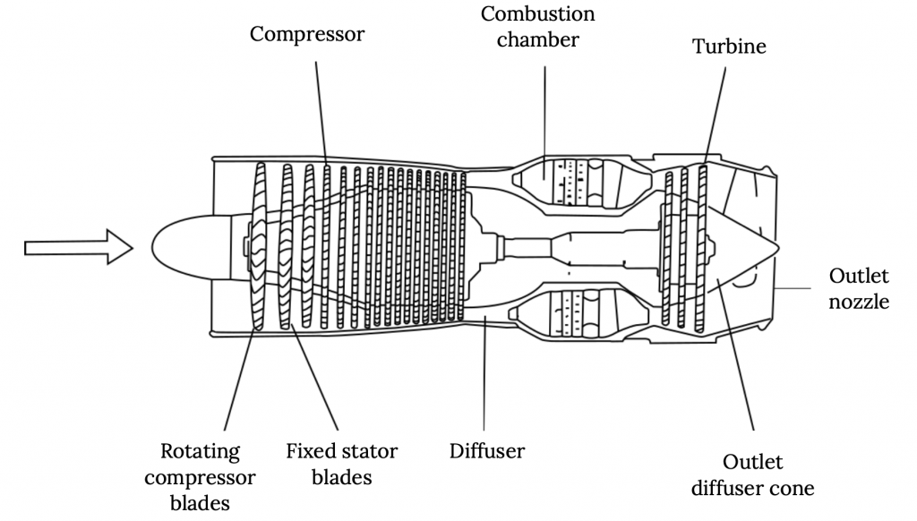
The most basic type of jet engine is called a “turbojet” and it consists basically of an inlet, followed by a compressor that increases the pressure (and lowers the speed) of the air before it enters the combustion chamber where fuel is added and ignited. After combustion a turbine extracts enough energy from the high energy (high speed) exhaust products to drive the compressor, and the flow then exits through the engine exhaust at high speed to provide thrust.

A cross-section of a turbojet engine shows how is is forced into increasingly smaller spaces. First air enters the engine and passes a set of rotating compressor blades. It next moves into a set of fixed stator blades immediately afterwards, before continuing into the rest of the compressor section, which continually narrows. The air then passes through a diffuser into a combustion chamber. After the combustion chamber, it passes through a turbine, where it is allowed to expand, and then the outlet nozzle, past the outlet diffuser cone in the center. — Figure 2.1: TurboJet Engine Illustration

It turns out that a pure turbojet isn’t a very efficient way to make thrust. It creates thrust through a very high speed exhaust and this is both very noisy and very loss prone. The high speed exhaust jet essentially rips its way through the surrounding air and this violent interaction between exhaust and atmosphere results in a lot of friction-like losses and makes a lot of noise.

We will look at jet propulsion in terms of momentum changes (energy per unit time) with the difference between the momentum in the exhaust and the engine inlet accounting for the thrust and, at first glance, it will seem that any way we can get a change in momentum is just as good as any other way, but that is not the case.

Momentum is essentially the mass multiplied by speed (velocity). This means that there are two ways to get a momentum change. One is to take a small amount of mass and accelerate it to a very high speed as is done in a turbojet engine. Another is to take a large amount of mass and accelerate it by a lesser amount. As it turns out, the latter way is the most efficient way to get thrust. It is sort of like comparing the effects of a large ceiling fan rotating slowly with those of a little “personal” fan. If you made two propeller driven air boats of the type used in swamps, one boat with a small propeller and the other with a large one, you would find that the boat with the larger prop would need less power to move at a given speed than the one with the small prop.

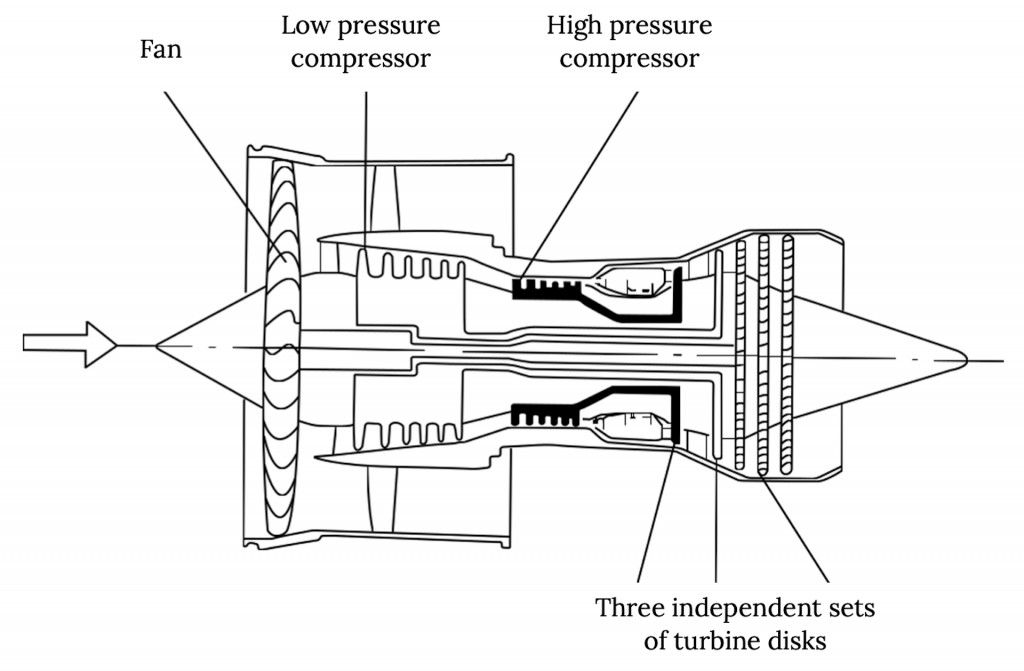
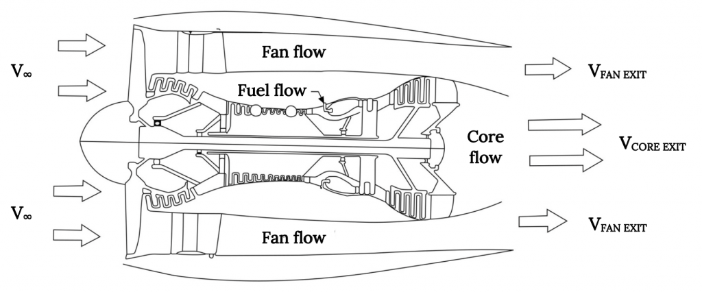
Fan-jets rely on this principle to provide more efficient thrust to an airplane than turbo-jets. In a fan-jet, the engine turbine or turbines drive both the compressor that works on the air going into the combustion chamber and a large fan that adds momentum to a large mass of air going around the engine core without being used to burn fuel. This fan or “bypass” air then mixes with the higher speed core, combustion products to give a high momentum total engine exhaust that derives its momentum from the large mass of the bypass flow and the high speed of the core flow.

A cross-section for a turbo-fan slash turbo-jet engine is shown. Air enters past the initial fan, with two paths afterwards: the outer edges bypassing the engine entirely and exiting the structure, and the central portions leading to a low pressure compressor, which then feeds into a high pressure compressor. After both compressors, air then basses through three independent sets of turbine discs before exiting out of the nozzle in the engine's rear. — Figure 2.2: Illustration of a Turbo-Fan or Fan-Jet Engine

So, for a given amount of thrust we will need a given amount of momentum change of the air going through the engine between its entrance and exit. We will look at how this momentum change mathematically accounts for the thrust a little later. The point here is that the most efficient way to get this momentum change with minimal losses is to accelerate a large mass of air by a small amount (small change in speed). This means that the bigger the bypass ratio (the ratio of the bypass air mass to the mass of air going through the engine core) the more efficient the engine is. But there is a limit to this.

As the fan jet engine gets larger due to higher bypass ratio design, the engine enclosure (nacelle) also gets larger and it produces more drag. So at some point it makes more sense to replace the bypass “fan” with a large propeller. The result is the “turboprop” engine.

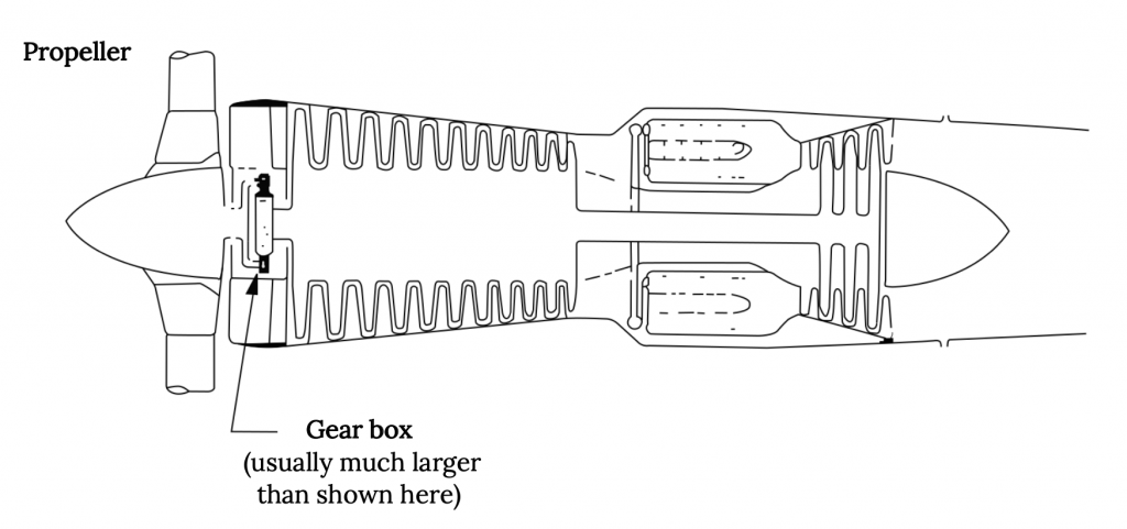
A turbo-prop engine's cross-section shows the propeller in front connected to a gear box in the center. The gear box is then connected to additional compressor blades, combustion chamber, and turbine fans, but these are not the main source of thrust. — Figure 2.3: Turboprop Engine Illustration

In the turboprop engine the flow through the engine core is really not used to produce any significant thrust. The exhaust turbine is designed to take all of the energy it can from the exhaust to drive the propeller and all of the engine’s thrust comes from the flow through the propeller. In a turboprop engine the amount of thrust that comes from the core flow is so negligible that, in some engine designs, the core flow actually goes “backwards”.

We might wonder, if the turboprop engine is more efficient than the fan-jet, which is in turn more efficient than the turbojet, why fan-jets are the engine of choice for most airplanes today? The answer is in the desired speed of flight.

Just as there is a big drag rise on a wing as it approaches the speed of sound, there are drag type losses on a propeller blade when its speed approaches Mach one. In fact, for a given propeller rotation speed, the limit on practical diameter for the prop is determined by the radius at which the propeller blade section reaches its critical Mach number. And, since the airspeed seen by the propeller blades is a function of both their rotational speed and the speed of the airplane, this limits the speed of the aircraft. Propeller design can extend this speed range somewhat with things like swept blade tips but the turboprop will always impose limits on aircraft cruise speeds.

Also, it turns out that the rotational speeds needed for a turboprop propeller are an order of magnitude below those of those in an efficient turbine core and this necessitates speed reduction gears between the turbine and the prop and this introduces both noise and vibrations that are not found in the fan-jet.

2.2 Propeller Engines

So what is the difference between a turboprop and a propeller driven by an internal combustion engine? From the point of view of the thrust provided by the propeller, there isn’t much difference. The difference is in the engine and the gearing that drives the propeller.

The turboprop is driven by a small turbine (jet) engine that sends as much of its energy as possible to the propeller through a driveshaft and reduction gear system. The IC engine propeller is attached to the driveshaft of an internal combustion engine that, like most automobile engines, uses the burning of gasoline or diesel fuel in a piston/cylinder type motor to turn the shaft.

Today most internal combustion driven propeller engines are found on smaller general aviation aircraft. This type of engine has provided reliable, affordable power for airplanes since the first flight of the Wright brothers in 1903. Over the years there have been many fascinating variations of IC engine used in airplanes, from the “rotary” engines of World War I in which the driveshaft was attached to the airplane and the propeller and engine actually rotated together around the shaft, to the massive piston engines of the 1940s and 1950s with dozens of cylinders arranged around the driveshaft like kernels on an ear of corn, to the four and six cylinder, car type but air cooled, engines usually found on today’s GA airplanes. These many varieties of IC engines would make an interesting and exhausting study in themselves, but that is beyond the scope of this text.

As far as we will be concerned, a propeller engine is a propeller engine, whether driven by a turbine or an IC engine or a rubber band. We will merely be concerned with the “power” output by the engine and we will call this the “shaft power” regardless of the type of engine that drives the shaft.

2.3 Thrust and Power

This brings us to the main difference in the way we will talk about propulsion for jet and prop engines. For jet powered aircraft, whether turbojets or fanjets, we will characterize the propulsion properties of the airplane in terms of thrust. For propeller powered airplanes, whether the propeller is attached to an IC engine or a turbine, we will talk about performance in terms of power.

Power and thrust are merely two different ways of looking at aircraft propulsion and performance. They are directly related to each other through speed.

Power = (Thrust)(Velocity)

While we normally talk about jet propulsion in terms of thrust and propeller propulsion in terms of power, there is little reason beyond convention that we must do so. We could talk about the power of a jet engine and the thrust of a propeller and we sometimes do so. Perhaps one reason for this distinction is that we will later find it convenient to look at the variation of both power and thrust with velocity and we will find that it is common to assume that thrust is fairly constant with speed for a jet and power is fairly constant with speed for a propeller driven plane.

The units normally associated with power and thrust, respectively, are pounds and horsepower. Yes, these are “politically incorrect” units; nonetheless, they are far more widely used than Newtons and Watts, their SI equivalents. [Have you ever heard anyone talk about the power of their car engine in watts?] This, of course, means we need to learn how the unit of horsepower relates to basic units in the “English” system.

1 horsepower = 550 foot-pounds / second.

[ A bit of engineering trivia: this conversion was used so often in the days of slide rule calculations that most slide rules had a special mark on them at the 550 location on the slide.]

2.4 Thrust and Conservation Laws

To find out how things like altitude and airspeed affect thrust and power we need to take a look at how the air goes through the propeller or the jet engine when an airplane is in flight and how the momentum of the air changes as it follows that path. To do this we will need to look at two “conservation laws”, conservation of mass and conservation of momentum.

2.4.1 Mass Conservation

In its simplest concept mass conservation is often stated something like “mass cannot be either created or destroyed; i.e., it is constant or conserved”. This is often accompanied by a qualifier noting that, in an atomic reaction, mass can actually be created (fusion reaction) or destroyed (fission reaction). This is an interesting way to look at mass if one is looking at the mass in the universe or in a closed container but it doesn’t help us when talking about engines. We need to look at the conservation of mass in a flow; that is, in the air going through a room or a pipe or a propeller or a jet engine.

If we had a sealed room filled with air it would be simple to state that the amount of air in the room is a constant. We could have people and plants in the room with the chemical reactions that are part of human breathing and plant chemistry continually altering the chemical constituencies in the “air”; nonetheless, the total mass of the “air” would remain constant.

The picture changes when we add ventilation to the room, either by using a forced ventilation system such as an air conditioning or heating system or by simply opening windows and doors. With either system there would be new air coming into the windows, doors, or intake vents and old air going out of other windows, doors, or exhaust vents. If we had a room with only a forced air inlet and no exhaust, the mass of air in the room would increase as air came in through the inlet. To accommodate this increasing mass the room would either have to expand like a balloon or the pressure and density of the air in the room would have to increase. Note that, if we assumed that the air was “incompressible” it would be impossible to pump new air into the room without providing an exhaust for an equal amount of air to escape. This would require conservation in the mass of the air in the room.

So in the example of room ventilation, conservation of mass for the air in the room would simply mean that, as a mass of new air enters the room, the same amount of mass of air must leave the room. Room or window air conditioners work this way, taking a given mass flow rate from the room, sending it through cooling coils, and returning that same mass flow rate to the room after some heat was removed from the air.

This brings us to the subject of mass flow rate, often called “m-dot” and given the symbol of a lower case “m” with a dot on top of the letter to represent a time derivative of the mass; i.e., mass per unit time, dm/dt.

When we speak of a room with vents or doors and windows we must talk about mass flow rates, and we say that in order to have mass conservation we must have no change in the mass within the room per unit time, simply another way of saying that the amount of mass that goes in during a given time period must equal the amount of mass that goes out in that same time. This is stated as:

dm/dt = 0 .

In other words, the amount of mass in the room does not change with time.

We often put this in equation form, saying that

dm/dt = Σ ρVA = 0.

Here, we are saying that the mass flow rate is equal to the density of the air, multiplied by its speed, as it passes through an area of size “A”. In other words, if air at sea level density is blowing through a window at a speed of 20 feet-per-second and if that window has an opening of 2 feet by 4 feet, we can calculate the mass of air per unit time that is passing through the window.

dm/dt = ρVA = (0.002378 sl/ft³)(20 ft/sec.)(2 ft x 4 ft) = 0.3805 sl/sec.

[Note here that the units of mass rate of flow have been found to be slugs per second. In the SI system they would be found in kilograms per second and in a version of the “English” system often used in fields such as Mechanical Engineering the units of mass flow rate would be pounds-mass per second.]

Now, if conservation of mass is met for the air in the room, the same mass of air per unit time must be going out of another opening or openings.

(dm/dt)_in + (dm/dt)_out = 0

(ρVA)_in + (ρVA)_out = 0

So, if there is a single window letting in the air flow found above and the exit is through a door, we can use conservation of mass to determine the speed of the air going out the door.

(ρVA)_out = – (ρVA)_in .

Just as three factors, the size (area) of the window, the speed of the air flow through the window, and the density of the air, determined the “mass flow rate” of the air coming into the room, the same three things determine the exit mass flow rate. In reality, all three of these things could be different at the exit (door, in this case), so, if we want to find the speed of the exiting air we must know both the area of the door and the density of the air at the door. However, there is no reason why the air flowing through the room would have changed density so we are safe in assuming “incompressible” flow, that is, density is constant. This gives us a simple equation:

(VA)_out = – (VA)_in .

So, if the door is 3 feet wide by 7 feet high, giving an area of 21 ft², while the window had an area of 8 ft², the speed of the air going out the door is:

V_out/V_in = – A_in/A_out

V_out = – V_in(A_in/A_out)

or in this case,

V_out = – 20 ft/sec. (8 ft² / 21 ft²) = – 7.62 ft/sec.

Now, why is there a minus sign with the exit velocity? This is because we, for no real reason, chose to give a positive sense to the velocity going in the window and since velocity is a vector; i.e., it has a direction, we have designated the flow of air into the room as positive. This means that the negative sign on the exit air velocity tells us it is going out of the room. While this may seem like an un-needed complication here, there are cases where it can help us figure out what is happening.

For example, suppose there are five windows and two doors in our room and we are told that air is coming into all five windows at a certain speed and is going out one door at a given speed, what is happening at the other door? Is the flow through that second door going into or out of the room?

We would have to write the complete equation for mass flow conservation to find both the amount and direction of the flow through the second door.

(ρVA)_w₁ + (ρVA)_w2 + (ρVA)_w3 + (ρVA)_w4 + (ρVA)_w5 – (ρVA)_D1 + (ρVA)_D2 = 0 .

Note that we have assigned positive values to the flow through all the windows since we were told that the flow was coming into all of them. We have also assigned a negative value to the flow out the first door since the flow was said to be out of that door. Also note that we did not assign a sign (direction) to the flow through the second door because we have no idea which way it is going. Now, if we put all the needed information for the five windows and first door into the terms in the equation and if we know the area of the second door and assume that density is the same everywhere (incompressible flow), we can solve for the speed (velocity) of the flow using the mass conservation relationship above and find both the magnitude of the speed and its direction (sign).

Exercise 2.1

Try doing the above problem assuming that all five windows are 2 ft X 4 ft in size and that air is blowing in at 20 ft/sec.

Assume that the two doors are both 3 ft X 7 ft in size and that the flow out of the first door is measured at 50 ft/sec.

Find the speed and direction of the flow through the second door.

NOTE: Here we considered all flow INTO our “system” or “control volume” as POSITIVE, and all flow OUT of the system as NEGATIVE. If we do not know its direction, we assume it is positive in value and the solution of the equation will give us a negative answer if we assumed the wrong direction. Later, when we look at the Momentum Equation we will use a unit vector, n, to assign a positive direction within our chosen axis system for flow through an opening, and that unit vector will always point OUT of the system.

OK, that was simple enough, but how do we deal with mass conservation when we are looking at flow through a jet engine or a propeller?

Mass conservation through a propeller or a jet engine works just like mass conservation in a flow going through a room. In fact, for the jet engine it is even simpler than the average room because there is only one well defined entrance and exit, or is that really the case?

A cross-section of a turbo-jet engine shows airflow entering at velocity cpa V sub infinity must first pass through several sets of compressor blades as it is compressed into smaller and smaller areas. It is then sent past the combustion chamber where the fuel flow controls the rate fuel is added for combustion. The air then expands through a set of turbine blades, exiting the exit nozzle at velocity cap V sub exit. — Figure 2.4: Mass Flows for a Turbo-Jet Engine

Technically, there is a second source of incoming mass in any jet engine and that is the mass flow of fuel coming into the engine. There is air coming into the engine inlet of a known area at (supposedly) a known speed and density, but the flow going out of the engine isn’t really just air, it is the gas that comes from combustion of the incoming air and the incoming fuel. The mass rate of flow coming out of the exit must account for both the mass of the entering air and the entering fuel, so our mass conservation relationship must recognize this.

(dm/dt)_inlet + (dm/dt)_fuel + (dm/dt)_exhaust = 0

We would normally write this as:

(ρAV)_inlet + (dm/dt)_fuel = – (ρAV)_exhaust .

So we must know the mass flow rate of the fuel. Usually the mass flow rate of the fuel is very small compared to that of the inlet air so perhaps that term can be neglected. So what’s the big deal? If we can neglect the fuel flow rate we are back to the one window, one door example and life is easy. Unfortunately there is another factor that we must not forget and that is density. Usually the flow through the exhaust of a jet engine is going pretty fast, near or greater than the speed of sound; i.e., we can no longer assume that density is constant as we did in the room ventilation example.

To solve this problem we have to know either the exit flow density or its speed in order to solve the equation for the “other” parameter (exit speed of density), and since the fuel mass flow contributes to this exit density we probably should not assume it to be negligible even if its velocity is almost negligible.

Making mass conservation for a jet even more complex is the fact that most of today’s jets are “fan jets” where there are essentially two entrance flows, one that goes through the engine core, mixing with the fuel to form a high speed exhaust, and another, larger, flow that is accelerated through the fan. We might analyze this problem by accounting for two separate entrance flows and two separate exit flows, or by assuming (correctly in most cases) that the two exit flows mix before leaving the engine covering or “nacelle” to form a single, mixed exhaust.

A cross-section of a fan-jet engine shows that air entering at velocity cap V sub infinity has two paths to take. The outer edges pass the fan and continue uninterrupted out of the back of the engine at velocity cap V sub fan exit. The central portions move through a set of compressor fans into a combustion chamber where the fuel flow determins how much is added for combustion. The air then passes through the turbine fans and exits as the core flow, with velocity cap V sub core exit. — Figure 2.5: Flows Through a Fan-Jet Engine

In any case, the jet engine flow problem is a little simpler for many people to understand than the propeller flow problem because the entrance and exit areas are normally pretty well defined. How do we define entrance and exit flows when we draw the flow through a propeller?

When a flow is going through a propeller, just what are the entrance and exit areas? There really is no physical entrance or exit. Of course, we know the flow goes through the propeller itself, so, is the propeller area used for both the flow “entrance” and its “exit”? This hardly makes sense. How can we talk about the changes in the flow between the entrance and exit when there is no physical distance between the entrance and exit?

Let’s look at what we know intuitively about the flow through a propeller (or a fan). We know that the flow behind the propeller or fan is moving faster than the flow in front of it. We know that in some way, a way that can be analyzed in detail by looking at each propeller or fan blade as a little rotating wing that does work on the air, the propeller essentially adds energy to the flow. We also know, if we think about it a bit, that we cannot use Bernoulli’s equation to compare the flow upstream and downstream of the prop or fan because energy is added at the prop or fan and Bernoulli’s equation assumes that energy is constant through the flow. We also know that there are limits to what a fan or propeller can do to accelerate a flow due to tip speed limits on the blades themselves and these limits essentially mean that we can pretty safely assume incompressible flow through the system.

Putting all these facts together, we can draw a picture that looks something like the flow should appear through a propeller or fan. We know that somewhere upstream of the propeller the flow is undisturbed; i.e., it is at “free-stream” or atmospheric conditions. We know that somewhere downstream of the prop the static pressure in the mass of air that went through the propeller must return to its free-stream value.

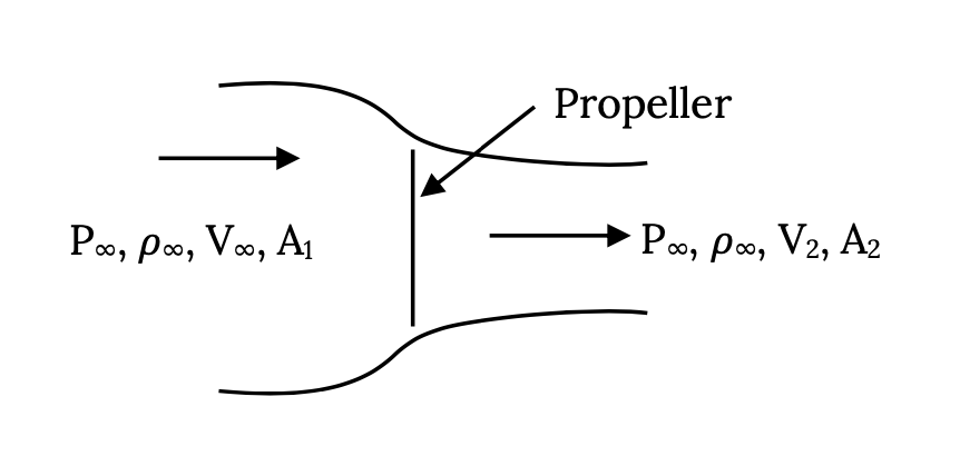
We will imagine a “stream-tube”, or three-dimensional path of constant mass flow, that starts out in the undisturbed flow upstream of the prop, goes through the prop (becoming the same diameter as the prop at that location, and then continues downstream until the point we mentioned above where the static pressure has returned to the atmospheric value. What must that “stream-tube” look like?

A stream-tube is defined as a three-dimensional flow path in which the mass flow rate is the same at every point along its journey. Essentially, as shown in the following figure, the upstream cross sectional area of the stream-tube (its “capture” area) must have the same amount of mass flow rate through it as goes through the prop itself. Likewise, the “exit” area for our stream-tube must also allow passage of the same mass flow as went through the capture area and the prop “disk” area.

As the relative flow approaches the propeller, the stream tubes narrow to match the propeller's width, then continue to narrow after passing it. This narrowed area results in a slipstream of faster-moving air inside the stream tube, while the surrounding flow is slower. — Figure 2.6: The Stream-tube Concept for a Propeller Flow

So why is the “stream-tube” in the figure above getting progressively smaller as the flow goes from the atmospheric pressure, free-stream capture area to the atmospheric pressure exit area somewhere downstream? First, we know the velocity in the exit area must be larger than in the capture (inlet) area; hence, if mass flow rate is the same and the flow is incompressible, the area must decrease in inverse proportion to the speed increases. But why do we assume that this area decrease (and speed increase) is smooth and continuous? Isn’t there simply a big jump in speed across the propeller disk?

Well, we probably could analyze everything in terms of some kind of instantaneous jump in flow speed at the propeller disk based on an energy balance, assuming that the energy added by the prop produces a sudden increase in flow kinetic energy and speed. However, we know from real world measurements that this speed increase is not instantaneous and that part of the increase is seen in front of the propeller as the flow speeds up from its “free-stream” velocity to the velocity right at the front of the prop disk. We also know that it takes a couple of propeller diameters downstream before the flow in the “propwash” reaches top speed. Based on this combination of reality and convenience, we choose to model the speed increase as a continuous one within a “stream-tube” shaped like a converging nozzle of circular cross section, as shown in the figure above.

This ideal picture, of course, ignores a lot of things such as the losses due to turbulence and rotational flow effects; nonetheless, it is one that works fairly well. So, what do we propose to do with this model and with the model of the flow through a jet engine? What we want to do is use these to determine how thrust is produced and find the properties that determine how thrust varies with speed and altitude.

2.4.2 Thrust

Our goal is to take a look at propulsion. How do we account for thrust or power in aircraft performance evaluations?

There are two ways to do this. One would look at energy additions to the flow and a conservation of energy. But, as noted in the propeller discussion above, this would be very tedious, requiring us to do aerodynamic analyses of each propeller blade, accounting for losses due to compressibility effects near the blade tips and for the interference between the flow over one blade and the following blade. There are books on how to do this, the oldest of which went under titles such as “Airscrew Theory”, and this is the type of analysis that companies making propellers must use. The problem would be even more interesting in a jet engine with us having to account for energy gains and losses due to flow around compressor blades and turbine blades, combustion of fuel, and flow though internal nozzles.

It turns out that the simplest way to look at thrust is to look at momentum conservation.

2.4.3 Momentum conservation

Momentum conservation, like mass conservation and energy conservation, is one of the “big three” conservation “laws” that we all saw somewhere back in some Physics course. On the face of it, conservation of momentum is a simple concept. Just as in mass conservation of a flow we must account for all mass flows that enter or leave the flow-field under consideration, in looking at momentum conservation we must consider all things that could possibly account for momentum changes and, ultimately, in forces.

Essentially, the concept we are looking at is one that says that the change of momentum in a body or “system” with time must equal the forces on that body or system. The idea is that either forces on a body or system will cause its momentum to change or a momentum change within the system or body will result in a force.

(d/dt)(momentum) = (d/dt)(mv) = Force

This is a simple idea that is often made to look very complicated when derived in most textbooks on fluid mechanics. If, for example, you kick a soccer ball, the force you impart to the ball will result in a change in momentum in the ball. If the ball was standing still before it was kicked, the force will change its momentum from zero to a value related to the force of the impact and the mass of the ball. If the ball was already moving, the kick may send moving in another direction, so this concept is directional; i.e., it is a vector concept, as would be expected when a force is involved.

In looking at aircraft propulsion we are interested in the reverse action; that is, creating a momentum change in order to get a force, changing the momentum of the flow through the engine or propeller to create thrust.

Just as in working with Bernoulli’s equation we had a choice of modeling the flow as a moving fluid going past a wing or body, or as a body moving through still air, we have to make a similar choice here. We will, for example, choose to look at the flow through a jet engine or a propeller as if the engine (prop) is standing still and the flow is moving past it. This is really a choice between having to consider the momentum of the moving engine or the momentum of the moving air. Either view will give the same answer for the thrust, but the moving air model is usually a little easier to work with. Either way, we must be very careful to account for all possible momentum changes in both the engine and the flow.

We first need to look at what kinds of momentum changes might be present as well as what kinds of forces might be involved. To do this, let’s look at one of the simplest of “jet” engines, but one of the hardest to analyze, a rubber balloon that is inflated and released.

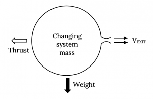
As the ballon's total mass changes due to the air exiting through the hole, the gas exits with a velocity cap V sub exit to the right, resulting in a net thrust force to the left. These are perpendicular to the balloon's downward weight force. — Figure 2.7: A Balloon as a Simple Jet

Let’s look at the illustration above and list all of the ways that momentum might play a role as well as all the forces involved. There will be at least two sources of change of momentum for the balloon and at least three forces that might be involved.

Momentum change sources:

The change in momentum of the balloon (the “system”) with time because of the change in mass of air inside the balloon with time and due to any changes in velocity of that mass. [As the balloon expels air through its inlet/outlet, the mass of the “system” itself is changing and, even if its speed was constant, the momentum of the system would change.]
The momentum of the flow exiting the “system” (balloon); i.e., the mass flow of air through the inlet/outlet (jet) multiplied by its velocity.

Both of these terms above are directional because of the velocities associated with them. The momentum of the balloon itself is related to the balloon’s velocity and the momentum of the flow through the exit is obviously related to the direction of the flow through the exit.

Forces on the balloon:

The major force on the balloon will be the one we choose to call thrust. This is essentially what we are trying to find.
nother force on the balloon that we might not think of at first is that due to gravity; i.e., its weight.
Finally, there would be any pressure forces caused by pressures acting on areas. These might include pressure drag on the balloon itself or differences in pressure across system boundaries. Often we find that pressure forces tend to balance out or sum to zero but there are some cases where these must be considered.
We could also consider friction forces or even electromagnetic or other forces if we wished but we will limit ourselves to the first three forces mentioned above.

How do we describe each of these sources of momentum change or forces in a very general way? Let’s look at each of these listed above.

1. The change in momentum of the “system” with time involves the changes in both mass and velocity of the system:

d/dt [(mass)(velocity)] ,

and, since the system mass can be written as its density times its volume, we might look at this as

d/dt [(density)(volume)(velocity)]

2. The change in momentum due to the flow out of (and in general) into the system with time is essentially the mass rate of flow (dm/dt) across any entrances or exits multiplied by the speed at which that mass is passing through the entrance or exit areas. We know that the mass rate of flow is the density multiplied by both the velocity and the flow cross sectional area, so this term is expressed as:

(dm/dt)(velocity) = (density)(velocity)(area)x(velocity) .

3. The weight is just the mass (density x volume) multiplied by the acceleration of gravity.

(density)(volume)(g) .

4. The pressure forces are just pressures acting on an area:

(pressure)(area)

Now, to work with all these we need to put them together in the form of some kind of equation. The equation must essentially say that the momentum changes must be balanced by the forces involved. This can be thought of as forces causing momentum change (the soccer player’s foot kicks the ball) or momentum changes causing forces (the thrust from a released balloon). The equation that usually results from a much more formal derivation is a complicated looking, vector relationship called the momentum equation.

2.4.4 The Momentum Equation

$ddt∭RρV¯dR+∬sρV¯(V¯⋅n^)dS⏟momentum change in fluid=−Fe−∬Sρn^ds+∭Rρg¯dR⏟Forces causing momentum change$

Before you panic at the vector notation and the double and triple integrals, take a deep breath and see how these terms relate to the ones presented above.

A triple integral over “R” (the mathematical “region” or the “system”) is nothing but the volume. If the density and velocity of everything contained in the region or system is the same; i.e., if it is a homogeneous system, then this term is nothing but the time derivative of the density times the volume times the velocity; i.e., of the system mass times its speed as it was stated in the section above.

So why do we make it so complicated looking? One reason might be just to impress our friends in liberal arts or to show our parents how hard our courses are. A better reason is to allow the momentum equation to account for non-homogenous system effects. Suppose, for example, that our “system” was not a balloon filled with nice homogenous air, but a baseball or golf ball with a solid filling made of several layers, each with different densities, and further, that someone had made the ball with its heavier core somewhat “off center”. You can buy such “trick” golf balls at novelty shops and when you hit them with a golf club (impart a force to the system!), instead of traveling in a straight line they wobble around as if they were drunk. Because the momentum equation can account for this “non-homogeneity” it can account for the wobbly motion of the trick golf ball. In a similar way the last term on the right, the gravity or weight term, can account for gravitational effects on a non-homogeneous mass.

Two of the terms in the equation have double integrals. You might have guessed by now that the double integral over a distance “S” must relate to some kind of area, and looking at the terms would confirm that. The double integral term on the left relates to the momentum carried with a flow into or out of the system over an entrance or exit area. This term is written in this complex way to be able to account for non-uniform velocities over the entrance or exit and even for non-uniform densities over these areas. If we assume that all of the entrance or exit flow is the same fluid moving at the same speed then the density and velocity terms can come outside the integral and the integral itself becomes nothing but the entrance or exit area. So, again, why make it look this complicated? Well, in many cases the flow out of an opening is not uniform because friction forces cause it to move more slowly near the edges of the opening than at the center, and this comprehensive form of the momentum equation can account for that if we want it to do so. Similarly, the pressure term on the right hand side of the equation can account for pressure variation over a surface.

What about the vector notation, the V•n term, in the double integral term on the left? First, the momentum equation is a vector equation, meaning that each of the terms has a direction and the solution of the equation for a force such as thrust or drag will give both a magnitude and a direction for that force. Second, for one of the terms on each side of the equation, it is only the parameter “normal” to a defined surface or boundary that will cause a force and the “unit vector” n is used to designate that normal direction. We will always define the direction for this unit vector as pointing out of the system, even where the flow is coming into the system.

What then do these vector quantities mean? Each of the velocities can have up to three terms in them, one associated with each direction in a selected axis system. In the case of velocity in a conventional x, y, z axis system, we normally use the terms u, v, and w to designate the x, y, and z components of velocity, respectively. So we would write a velocity vector as:

V = ui + vj + wk ,

where i, j, and k are the unit vectors in the positive x, y, and z directions. In a similar manner, the gravity vector could have up to three components; however, we sometimes try to define our coordinate system so one axis is in the direction of gravitational acceleration to eliminate two of these components.

The V•n term is then the “dot product” of two vectors where both the V and the n vectors may have x, y, and z components, but only the like directed components multiply with each other, then sum to give a “scalar” quantity with a magnitude but no direction. So, if the velocity is in the same direction as the normal vector (as is often the case for flows into or out of a system) the result is simply the magnitude of the velocity. At the other extreme, if the velocity is at a 90 degree angle to the normal vector the dot product gives zero.

Again one might ask, why make things so complicated with all these integrals and vectors and dot products and the like? It is done this way because it is a very versatile equation that can account for fully three dimensional motion. For example, should that soccer player kick the ball at a 90 degree angle to its existing direction of motion, this relationship would, provided we knew the force of the kick and the mass and velocity of the ball, tell us the ball’s new direction and speed even though the direction would be in neither the original direction of motion or in the direction of the kick. Similarly, if there is a bend in a pipe we can use the equation to find the magnitude and direction of the force that will occur when water flows through that bend in the pipe.

The trick to using the momentum equation is to follow the rule of thumb that often distinguishes an engineer from a pure scientist or mathematician; that is to use proper alignment of axis systems and to set system boundaries and to make good assumptions that will eliminate as much of the complexity as possible. Fortunately we can do a lot of this as we use the momentum equation to look at thrust.

2.4.5 Thrust (again)

Let’s look at the flow through a jet engine in terms of the momentum equation.

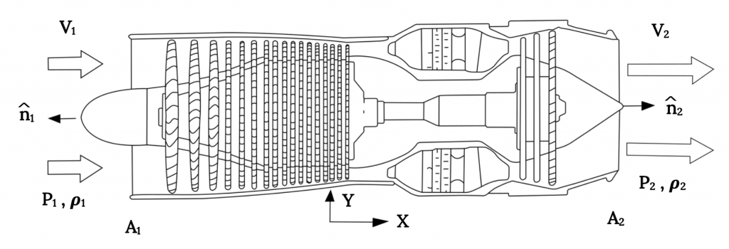
At the intake for the turbo-jet engine with an area of cap A sub 1, the normal points outward, to the left, while the air flowing into the engine at velocity cap V sub 1, pressure cap P sub 1, and density rho sub 1, enter to the right. At the exit with an area cap A sub 2, the normal points outward, to the right, aligned with the exiting air flow at velocity cap V sub 2, pressure cap P sub 2, and density rho sub 2. — Figure 2.8:Momentum Equation Terms for Turbo-Jet

In the illustration above we have aligned the engine with the “x” axis and we have flow coming into the engine inlet in the x direction and another flow coming out of the engine, also in the x direction. We want to know the thrust as a function of this information. Let’s look at what we can say about the various terms in the momentum equation.

The first term on the left hand side of the equation is a “time dependent” term to account for changes in momentum of the “system” itself with time. Here our system is the entire jet engine, and, if we assume that the engine (airplane) is in “steady” or constant speed flight, there is nothing in the term (density, velocity, or volume) that is changing with time. So, this term is zero.

The second term on the left accounts for the momentum carried into or out of the system as flow enters or leaves. Obviously, this term will not go away since we have air coming into the engine and combustion products going out the other end. First we need to ask if these two flows are “uniform” across their respective entrance or exit areas. If we can assume that they are uniform and can assume that all of the flow has the same density, then this term (actually two terms, one for the entrance and one for the exit) becomes:

ρ₁V₁(V₁•n₁)A₁ + ρ₂V₂(V₂•n₂)A₂ .

Now, what do we do with the vector business? The flows are both in the positive x direction. The first normal unit vector is in the negative x direction while the second is in the positive x direction. The result is:

– ρ₁V₁²A₁ + ρ₂V₂²A₂ , (all in the x direction)

Ok, that takes care of the left hand side of the momentum equation. What happens to the terms on the right? The first term on the right is the “external” force which, in this case, is the thrust we want to find. The second term on the right is perhaps the hardest to understand physically so we will come back to this.

The third term on the right is the gravity term, really the weight. If we assume that this is acting at a 90 degree angle to the x axis or the direction of flight and thus is perpendicular to all the other forces and momentum changes in which we have an interest we might simply neglect this term. Actually it would be more proper to say that its component in the x direction is zero. In reality, this term would tell us that there must be a force to oppose the weight and this would be the aerodynamic lift which, in turn, would be related in the momentum equation to a vertical change in momentum of the flow as it moved around the wing and the corresponding pressure distribution around the wing. In essence we are choosing to ignore the vertical components of the forces and momentum changes.

Now let’s go back to the second term on the right, the only term with pressures in it. This term looks at forces caused by pressures acting on areas. If we were looking at the lift force we would use this term to integrate the pressure distribution around a wing. On the engine we will assume that the flows over the outside of the engine casing or nacelle are symmetrical, that is that the same pressure distribution exists on the top as on the bottom of the nacelle, and that the net effect of these pressures (at least in the x direction) is zero. But what about pressures across the entrance and exit?

Pressures across the entrance and exit?!! How can this mean anything when there are no real surfaces here, just flows going in or out? This is where the concept of a “system” boundary gets interesting. When there is a real boundary such as the engine nacelle the bounds of the system are easy to understand. But these “open” ends of the “system” are also boundaries over which we must account for all the terms in the equation. In other words, just as we had to account for the flow through these somewhat imaginary boundaries, we must also account for pressure changes across them. But how can these pressures cause real forces when there are no “real” surfaces for them to act on? This becomes one of those “leaps of faith” that we often must take in applying equations to physical situations.

No, there are no surfaces at the entrance and exit where the pressure differences across the surface cause a force; however, we must account for them anyway if there is a pressure differential between the surrounding atmosphere and the flow into the entrance and out of the exit. This is probably the easiest to understand when we look at the exhaust flow.

Coming out of the exhaust is a flow of the combustion products of air and fuel that has been heated and pressurized in the engine combustor. After combustion we want to turn that added energy into as high a momentum (the second term on the left hand side of the momentum equation) as possible. This means that we want to “expand” the gas in a exit nozzle, lowering its pressure with a corresponding increase in speed (ala Bernoulli’s equation) as much as possible to get a high momentum. The ideal situation is to expand it to the point where the exiting gas has the same pressure as the atmosphere into which it will exit. If it expands too much or too little there will be losses as the flow pressure comes to equilibrium with the atmosphere. It turns out (and the momentum equation essentially tells us this) that the losses from over or under-expansion are equivalent to the pressure force that would be on a surface with the same area as the exit with a pressure difference equal to that under or over-expansion delta-P. This is why some high performance jets have variable area exit nozzles on their engines.

The same problem can occur to a lesser degree at the engine inlet but a properly designed engine inlet and compressor section can eliminate most of the loss.

So, how do we deal with this pressure term? We either must know the differences between the atmospheric pressure and those of the entrance and exit flows and compute values for these terms, being careful to account properly for the unit vector signs, or we must assume that these losses are negligible. Let us take the easy way out and assume that these terms are of little consequence because we have a properly designed engine.

OK, where does this leave us? We have ended up with a relatively simple equation:

– ρ₁V₁²A₁ + ρ₂V₂²A₂ = – Fe

rearranging this gives:

Thrust = Fe = ρ₁V₁²A₁ – ρ₂V₂²A₂ .

Looking at this we see that the second term on the right will be much greater than the first term, so, the thrust will have a negative sign. Is this ok? Sure it is. It just says the thrust force is in the negative x direction, toward the left, just as we want it to be.

Wow! That sure was a lot of work to get a fairly obvious answer; the thrust is equal to the momentum change from engine inlet to exit! Isn’t this somewhat intuitive? Yes, it sortof is intuitive to many of us. On the other handit does keep the mathematicians and theoreticians in our midst happy, and more importantly, it tells us that in arriving at this “intuitive” answer we have made some important assumptionsabout pressure behavior and axis system selection, etc.

Ok, now that we have all that under our belts what important facts about propulsion can be drawn from this solution? To see this, let’s play around with the equation above a little by accounting for conservation of mass.

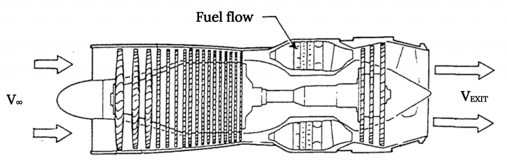
Now, recognizing that V₁ is our “free stream” speed, V_∞, and that the entering air density is also that of the atmosphere, ρ_∞, we can write this as

Thrust = ρ_∞V_∞²A₁ – ρ₂V₂²A₂

And looking only at the magnitude of the thrust (as said above, the relationship above gives a negative thrust, signifying simply that it is to the left in our original illustration of the engine moving from right to left)

Thrust = ρ₂V₂²A₂ – ρ_∞V_∞²A₁

We now define the “static thrust” as T₀, the thrust when the engine is standing still (V_∞ = 0). This is the amount of thrust that would be measured on an engine test stand and is a standard piece of information that would exist for any engine.

T₀ = ρ₂V₂²A₂

This allows us to rewrite the general thrust relationship as:

Thrust = T₀ – ρ_∞V_∞²A₁ ,

or simply as:

T = T₀ – a V_∞² ,

where:

a = ρ_∞A₁

What does all this tell us? First, all the thrust equations tell us that thrust is a function of the atmospheric density. Unlike velocity, which we earlier found to vary with the square root of density, thrust decreases in direct proportion to the decrease of density in the atmosphere. Thus, we write:

T_alt = T_sl(ρ_alt/ρ_SL)

This is an important relationship between thrust and altitude that we will use in all performance calculations.

Second, we learn that, in general, the thrust of an engine varies with speed according to the relationship:

T = T₀ – a V_∞²

It should be noted, as always, that these equations involve important assumptions, such as the assumption that engine exit pressure and entrance pressure are both equal to the pressure in the free stream atmosphere. Pilots of jet aircraft will tell you that the thrust to static thrust relationship shown above doesn’t, for example, account for an engine surge on initial acceleration down the runway as a “ram effect” into the engine inlet occurs. This “ram effect” is essentially one of these pressure effects that we chose to ignore.

2.4.6 Propeller Thrust

It should be noted that we would get essentially the exact same thrust equation looking at the flow through a propeller as we do with a jet engine. Keeping in mind an earlier discussion, we would draw our “system” as shown below using boundaries that represent a “stream tube” of constant mass flow. In this case we have no easy way of knowing the exact values for the entering flow area or the exit area but we would get exactly the same equation as we found for the jet and we would still find

T = T₀ – aV_∞².

Airflow approaches a propeller with pressure cap P sub infinity, density rho sub infinity, velocity cap V sub infinity, and area cap A sub 1. The air then exits past the propeller with the same pressure and density, but an updated velocity of cap V sub 2 and reduced area cap A sub 2. Thrust cap T is still shown to be equal to the static thrust cap T knot minus the speed of sound a times cap V sub infinity squared. — Figure 2.9:Momentum Equation Terms for Propeller Flow

In this chapter we have looked at the relatively simple models of aircraft propulsion that we will use in examining aircraft performance. In doing this we have used some basic physical concepts of conservation (mass and momentum), both of which can provide very powerful tools for evaluating forces and motions in fluid flows and other areas. We made a lot of simplifying assumptions along the way in order to understand some very basic concepts related to jet and propeller propulsion; in particular, to give a basis for modeling the way both thrust and power vary with speed and altitude. We will find these concepts very useful in later chapters.

Homework 2

1. In a wind tunnel the speed changes as the cross sectional area of the tunnel changes. If the speed in a 6′ x 6′ square test section in 100 mph, what was the speed upstream of the test section where the tunnel measures 20′ x 20′? Use conservation of mass and assume incompressible flow. Conservation of mass requires that as the flow moves through a path or a duct the product of the density, velocity and cross sectional area must remain constant; i.e. that ρVA = constant.

2. A model is being tested in a wind tunnel at a speed of 100 mph.

(a) If the flow in the test section is at sea level standard conditions, what is the pressure at the model’s stagnation point?

(b) The tunnel speed is being measured by a pitot-static tube connected to a U-tube manometer. What is the reading on that manometer in inches of water.

References

Figure 2.1: Claire Colvin (2021). “TurboJet Engine Illustration.” CC BY 4.0.

Figure 2.2: Claire Colvin (2021). “Illustration of a Turbo-Fan or Fan-Jet Engine.” CC BY 4.0.

Figure 2.3: Claire Colvin (2021). “Turboprop Engine Illustration.” CC BY 4.0.

Figure 2.4: Claire Colvin (2021). “Mass Flows for a Turb-Jet Engine.” CC BY 4.0.

Figure 2.5: Claire Colvin (2021). “Flows Through a Fan-Jet Engine.” CC BY 4.0.

Figure 2.6: James F. Marchman (2004). “The Stream-tube Concept for a Propeller Flow.” CC BY 4.0.

Figure 2.7: Kindred Grey (2021). “A Balloon as a Simple Jet.” CC BY 4.0. Adapted from James F. Marchman (2004). CC BY 4.0. Available from https://archive.org/details/2.1_20210804

Figure 2.8: Claire Colvin (2021). “Momentum Equation Terms for Turbo-Jet.” CC BY 4.0.

Figure 2.9: Kindred Grey (2021). “Momentum Equation Terms for Propeller Flow.” CC BY 4.0. Adapted from James F. Marchman (2004). CC BY 4.0. Available from https://archive.org/details/2.9_20210804

<!– pb_fixme –><!– pb_fixme –>