
6: Range and Endurance
- Page ID
- 75450

\( \newcommand{\vecs}[1]{\overset { \scriptstyle \rightharpoonup} {\mathbf{#1}} } \)
\( \newcommand{\vecd}[1]{\overset{-\!-\!\rightharpoonup}{\vphantom{a}\smash {#1}}} \)
\( \newcommand{\dsum}{\displaystyle\sum\limits} \)
\( \newcommand{\dint}{\displaystyle\int\limits} \)
\( \newcommand{\dlim}{\displaystyle\lim\limits} \)
\( \newcommand{\id}{\mathrm{id}}\) \( \newcommand{\Span}{\mathrm{span}}\)
( \newcommand{\kernel}{\mathrm{null}\,}\) \( \newcommand{\range}{\mathrm{range}\,}\)
\( \newcommand{\RealPart}{\mathrm{Re}}\) \( \newcommand{\ImaginaryPart}{\mathrm{Im}}\)
\( \newcommand{\Argument}{\mathrm{Arg}}\) \( \newcommand{\norm}[1]{\| #1 \|}\)
\( \newcommand{\inner}[2]{\langle #1, #2 \rangle}\)
\( \newcommand{\Span}{\mathrm{span}}\)
\( \newcommand{\id}{\mathrm{id}}\)
\( \newcommand{\Span}{\mathrm{span}}\)
\( \newcommand{\kernel}{\mathrm{null}\,}\)
\( \newcommand{\range}{\mathrm{range}\,}\)
\( \newcommand{\RealPart}{\mathrm{Re}}\)
\( \newcommand{\ImaginaryPart}{\mathrm{Im}}\)
\( \newcommand{\Argument}{\mathrm{Arg}}\)
\( \newcommand{\norm}[1]{\| #1 \|}\)
\( \newcommand{\inner}[2]{\langle #1, #2 \rangle}\)
\( \newcommand{\Span}{\mathrm{span}}\) \( \newcommand{\AA}{\unicode[.8,0]{x212B}}\)
\( \newcommand{\vectorA}[1]{\vec{#1}} % arrow\)
\( \newcommand{\vectorAt}[1]{\vec{\text{#1}}} % arrow\)
\( \newcommand{\vectorB}[1]{\overset { \scriptstyle \rightharpoonup} {\mathbf{#1}} } \)
\( \newcommand{\vectorC}[1]{\textbf{#1}} \)
\( \newcommand{\vectorD}[1]{\overrightarrow{#1}} \)
\( \newcommand{\vectorDt}[1]{\overrightarrow{\text{#1}}} \)
\( \newcommand{\vectE}[1]{\overset{-\!-\!\rightharpoonup}{\vphantom{a}\smash{\mathbf {#1}}}} \)
\( \newcommand{\vecs}[1]{\overset { \scriptstyle \rightharpoonup} {\mathbf{#1}} } \)
\(\newcommand{\longvect}{\overrightarrow}\)
\( \newcommand{\vecd}[1]{\overset{-\!-\!\rightharpoonup}{\vphantom{a}\smash {#1}}} \)
\(\newcommand{\avec}{\mathbf a}\) \(\newcommand{\bvec}{\mathbf b}\) \(\newcommand{\cvec}{\mathbf c}\) \(\newcommand{\dvec}{\mathbf d}\) \(\newcommand{\dtil}{\widetilde{\mathbf d}}\) \(\newcommand{\evec}{\mathbf e}\) \(\newcommand{\fvec}{\mathbf f}\) \(\newcommand{\nvec}{\mathbf n}\) \(\newcommand{\pvec}{\mathbf p}\) \(\newcommand{\qvec}{\mathbf q}\) \(\newcommand{\svec}{\mathbf s}\) \(\newcommand{\tvec}{\mathbf t}\) \(\newcommand{\uvec}{\mathbf u}\) \(\newcommand{\vvec}{\mathbf v}\) \(\newcommand{\wvec}{\mathbf w}\) \(\newcommand{\xvec}{\mathbf x}\) \(\newcommand{\yvec}{\mathbf y}\) \(\newcommand{\zvec}{\mathbf z}\) \(\newcommand{\rvec}{\mathbf r}\) \(\newcommand{\mvec}{\mathbf m}\) \(\newcommand{\zerovec}{\mathbf 0}\) \(\newcommand{\onevec}{\mathbf 1}\) \(\newcommand{\real}{\mathbb R}\) \(\newcommand{\twovec}[2]{\left[\begin{array}{r}#1 \\ #2 \end{array}\right]}\) \(\newcommand{\ctwovec}[2]{\left[\begin{array}{c}#1 \\ #2 \end{array}\right]}\) \(\newcommand{\threevec}[3]{\left[\begin{array}{r}#1 \\ #2 \\ #3 \end{array}\right]}\) \(\newcommand{\cthreevec}[3]{\left[\begin{array}{c}#1 \\ #2 \\ #3 \end{array}\right]}\) \(\newcommand{\fourvec}[4]{\left[\begin{array}{r}#1 \\ #2 \\ #3 \\ #4 \end{array}\right]}\) \(\newcommand{\cfourvec}[4]{\left[\begin{array}{c}#1 \\ #2 \\ #3 \\ #4 \end{array}\right]}\) \(\newcommand{\fivevec}[5]{\left[\begin{array}{r}#1 \\ #2 \\ #3 \\ #4 \\ #5 \\ \end{array}\right]}\) \(\newcommand{\cfivevec}[5]{\left[\begin{array}{c}#1 \\ #2 \\ #3 \\ #4 \\ #5 \\ \end{array}\right]}\) \(\newcommand{\mattwo}[4]{\left[\begin{array}{rr}#1 \amp #2 \\ #3 \amp #4 \\ \end{array}\right]}\) \(\newcommand{\laspan}[1]{\text{Span}\{#1\}}\) \(\newcommand{\bcal}{\cal B}\) \(\newcommand{\ccal}{\cal C}\) \(\newcommand{\scal}{\cal S}\) \(\newcommand{\wcal}{\cal W}\) \(\newcommand{\ecal}{\cal E}\) \(\newcommand{\coords}[2]{\left\{#1\right\}_{#2}}\) \(\newcommand{\gray}[1]{\color{gray}{#1}}\) \(\newcommand{\lgray}[1]{\color{lightgray}{#1}}\) \(\newcommand{\rank}{\operatorname{rank}}\) \(\newcommand{\row}{\text{Row}}\) \(\newcommand{\col}{\text{Col}}\) \(\renewcommand{\row}{\text{Row}}\) \(\newcommand{\nul}{\text{Nul}}\) \(\newcommand{\var}{\text{Var}}\) \(\newcommand{\corr}{\text{corr}}\) \(\newcommand{\len}[1]{\left|#1\right|}\) \(\newcommand{\bbar}{\overline{\bvec}}\) \(\newcommand{\bhat}{\widehat{\bvec}}\) \(\newcommand{\bperp}{\bvec^\perp}\) \(\newcommand{\xhat}{\widehat{\xvec}}\) \(\newcommand{\vhat}{\widehat{\vvec}}\) \(\newcommand{\uhat}{\widehat{\uvec}}\) \(\newcommand{\what}{\widehat{\wvec}}\) \(\newcommand{\Sighat}{\widehat{\Sigma}}\) \(\newcommand{\lt}{<}\) \(\newcommand{\gt}{>}\) \(\newcommand{\amp}{&}\) \(\definecolor{fillinmathshade}{gray}{0.9}\)Introduction
A Little Background
In the earliest days of powered flight the primary concern was getting the aircraft into the air and back down safely (with safely meaning the ability to limp away after the “landing”). The Wright’s famous first flight was shorter than a football field and even for a couple of years after December of 1903 they were content to circle around the family farm The Wright’s home built engines couldn’t run for long periods of time and they simply didn’t envision the need or desire for flights over distances of over a few miles. In 1908, however, Scientific American magazine challenged aviation experimenters to produce an aircraft or “aero-plane”[1] which could fly, in public view, over a distance of one mile! While the Wright’s claimed to be able to make such a flight, their obsession with secrecy as they sought military sales and their egotistical belief that no one else could approach their expertise in aviation led them to ignore the prize offered by Scientific American for the one mile public flight.
It was Glenn Curtiss, a builder of motorcycle engines and holder of numerous world speed records in motorcycle racing, who, in July of 1908, made the first public one-mile flight. Curtiss, who had worked with Alexander Bell and others to develop their own airplanes, made the flight with newspaper reporters watching and with movie cameras recording the flight. Curtiss became the top aviator in America and the Wrights were furious, leading to numerous legal suits as Wilbur and Orville sought to prove in the courts that Curtiss and Bell had infringed on their patents. Curtiss went on to outperform the Wrights and others in aviation meets in America and Europe. The Wright’s subsequent patent suits aimed at reserving for themselves the sole rights to design and build airplanes in the United States stagnated aircraft development in America and shifted the scene of aeronautical progress to Europe where it remained until after World War I.
As aircraft and aviation continued to develop, range and endurance became the primary objective in aircraft design. In war, bombers needed long ranges to reach enemy targets beyond the front lines and by the end of World War I huge bombers had been developed in several countries. After the war, European governments subsidized the conversion of these giants into passenger aircraft. Some larger planes had even been built as passenger carrying vehicles before the conflict. Sikorski’s early designs are good examples. In the United States, however, with little government interest in promoting air travel for the public until the late 1920’s, long range aircraft development was more fantasy than fact. In 1927 Lindberg’s trans-Atlantic flight captured the public’s imagination and interest in long range flight increased. Lindberg’s flight, like that of Curtiss, was prompted by a prize from the printed media, illustrating the role of newspapers and magazines in spurring technological progress.
By the late 1930’s the public began to see flight as a way to travel long distances in short times, national and international airline routes had developed, and planes like the “China Clipper” set standards for range and endurance. World War II forced people and governments to think in global terms leading to wartime development of bombers capable of non‑stop flight over thousands of miles and to post‑war trans‑continental and trans‑ocean aircraft. Since 1903 we have seen aircraft ranges go from feet to non‑stop circling the globe and endurances go from minutes to days!
6.1 Fuel Usage and Weight
In studying range and endurance we must, for the first time in this course, consider fuel usage. In the aircraft of Curtiss and the Wrights, it was not uncommon for the engine to quit from mechanical problems or overheating before the fuel ran out. In today’s aircraft, range and endurance depend on the amount of fuel on board. When the last drop of fuel is gone the plane has reached its limit for range and endurance. One could, of course, include the glide range and endurance after the aircraft runs out of fuel, but an airline that operated that way would attract few passengers!
Fuel usage depends on engine design, throttle settings, altitude and a number of other factors. It is, however, not the purpose of this text to study engine fuel efficiency or the pilot’s use of the throttle. We will assume that we are given an engine with certain specifications for efficiency and fuel use and that the throttle setting is that specified in the aircraft handbook or manual for optimum range or endurance at the chosen altitude. It is assumed that the student will take a separate course on propulsion to study the origins of the figures used here for these parameters.
Our primary concern in fuel usage will be the change in the weight of the aircraft with time. Many of our performance equations used in previous chapters include the aircraft weight. In those chapters we treated weight as a constant. Weight is, in reality, constant only for the glider or sailplane. For other aircraft the weight is always changing, always decreasing as the fuel is burned. This means that the aerodynamic performance of the airplane changes during the flight. This does not, however, negate the value of the methods used earlier to study cruise and climb. Those calculations will normally be done using the maximum gross weight of the airplane which will lead to a conservative or “worst case” analysis of those performance parameters. We can also use the methods developed earlier to look at the “instantaneous” capabilities of the aircraft at a given weight, realizing that at a later time in flight and at a lower weight, the performance may be different.
In considering range and endurance it is imperative that we consider weight as a variable, changing from maximum gross weight at take‑off to an empty fuel tank weight at the end of the flight. To do this we will deal with fuel usage in terms of the weight of the fuel (as opposed to fuel volume, in gallons, which we normally use for automobiles). When our concern is endurance we are interested in the change in weight of the fuel per unit time
\[\dfrac{dW_f}{dt}\]
and, when range is the concern we want to know how the weight of fuel decreases with distance traveled.
\[\dfrac{dW_f}{dS}\]
Aircraft engine manufacturers like to specify engine fuel usage in terms of specific fuel consumption. For jet engines this becomes a thrust specific fuel consumption and for prop aircraft, a power specific fuel consumption. Since thrust and power bring different units into the equations we must consider the two cases separately.
6.2 Range and Endurance: Jet
We speak of the engine output of a jet engine in terms of thrust; therefore, we speak of the fuel usage of the jet engine in terms of a thrust specific fuel consumption, Ct. Ct is the mass of fuel consumed per unit time per unit thrust. The unit of time should be seconds and the unit for thrust should be in pounds or Newtons of thrust.
[Ct] = (sl/sec)/lbthrust , or = (kg/sec)/Nthrust
The above is the proper definition of thrust specific fuel consumption, however, it is not really exactly what we need for our calculations. We would prefer a definition based on weight of fuel consumed instead of the mass. We will thus define a weight specific fuel consumption, t, as the weight of fuel used per unit time per unit thrust. This gives units of (time)-1.
\[\left[\gamma_{\mathrm{t}}=\mathrm{gC}_{\mathrm{t}}\right]=\left(\mathrm{lb}_{\text {fuel }} / \mathrm{sec}\right) / \mathrm{lb}_{\text {thrust }}, \text { or }=\left(\mathrm{N}_{\text {fuel }} / \mathrm{sec}\right) / \mathrm{N}_{\text {thrust }}=(\mathrm{sec})^{-1}\]
The reader should be aware that many aircraft performance texts and propulsion texts are very vague regarding the units of specific fuel consumption. Some even define it in terms of mass and give it units of 1 / sec., making it dimensionally incorrect. Part of the confusion, particularly in older American propulsion texts, lies in the use of the pound‑mass as the unit of mass. This gives a combination of pounds‑mass divided by pounds‑force, which, in reality gives sec2 / ft. The situation is then further complicated by the author seemingly throwing in a term called gc which is supposed to resolve the lbm /lbf issue. At any rate it is very important that the engineer using specific fuel consumption carefully consider the units involved before beginning the solution of a range or endurance problem. A correctly specified weight specific fuel consumption will have units of sec-1 and will do so without the use of anything called gc.
It should be added that one might also encounter specific fuel consumption which has been calculated using mass of fuel (kg) and thrust in kilograms, a non-SI unit which is used in much of the world (virtually no one in the world knows what a Newton is or how to use it). If this is done the numerical value should be the same as obtained using the weight specific fuel consumption definition above.
Some sources of specific fuel consumption data use units of (hours)-1 since the hour is a more convenient unit of time. The use of seconds is, however, correct in any standard unit system and the student may be well advised to convert hours to seconds before beginning calculation even though this will ultimately result in the calculation of endurance in seconds, giving rather large numbers for answers.
To find endurance we want the rate of fuel weight (Wf) change per unit time which can be written in terms of the thrust specific fuel consumption
\[\mathrm{dW}_{\mathrm{f}} / \mathrm{dt}=\gamma_{\mathrm{t}} \mathrm{T}\]
And, in straight and level flight where thrust equals drag
\[\mathrm{d} \mathrm{W}_{\mathrm{f}} / \mathrm{dt}=\gamma_{\mathrm{t}} \mathrm{D}\]
For maximum endurance we want to minimize the above term. This clearly shows that for maximum endurance the jet plane must be flown at minimum drag conditions. We will look at how to find that endurance after taking a brief look at range.
To find the flight range we must look at the rate of change of fuel weight with distance of flight. We might pause a little at this point to realize that this may be more complicated than endurance because range will depend on more than simply the aerodynamic performance of the airplane. It will also require consideration of the wind speed. An airplane can fly forever at a speed of 100 mph into a 100 mph head‑wind and still have a range of zero! For now, however, we will put those worries aside and look at the simple mathmatics with which we begin consideration of the problem. We looked above at the rate of weight change with time. We can combine this with the change of distance with time (speed) to get the rate of change of weight with distance.
\[\mathrm{dW}_{\mathrm{f}} / \mathrm{dS}=\left(\mathrm{dW}_{\mathrm{f}} / \mathrm{dt}\right) /(\mathrm{dS} / \mathrm{dt})=\gamma_{\mathrm{t}}(\mathrm{T} / \mathrm{V})=\gamma_{\mathrm{t}}(\mathrm{D} / \mathrm{V})\]
Note that we still assume D = T or straight and level flight.
From the above it is obvious that maximum range will occur when the drag divided by velocity (D/V) is a minimum. This is not a condition which we have studied earlier but we can get some idea of where this occurs by looking at the plot of drag versus velocity for an aircraft.
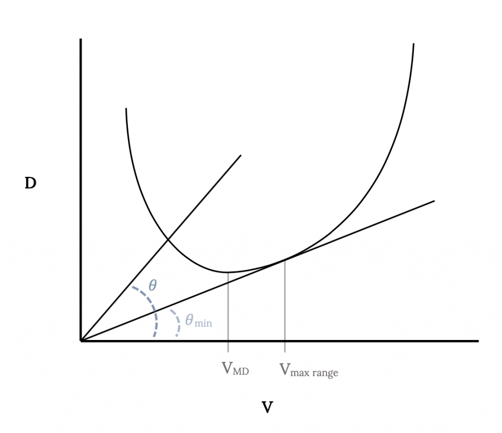
On this plot a line drawn from the origin to intersect the drag curve at any point has a tangent equal to the drag at the point of intersection divided by the velocity at that point. The minimum possible value of D/V for the aircraft represented by the drag curve must then be found when the line is just tangent to the drag curve. This point will give the velocity for maximum range. Note that it is a higher speed than that for minimum drag (which, in turn was higher than the speed for minimum power).
In the above we have found the conditions needed to achieve maximum range and endurance for a jet aircraft. We have not yet found equations for the actual range or endurance. To find these we need to return to the time and distance differentials and integrate them. For time we have
")
We now wish to put the equations in a form which includes the weight of the aircraft instead of the weight of the fuel. Since the change in weight of the aircraft in flight is equal and opposite the weight of fuel consumed
dW = – dWfuel
we have
")
Finally, integrating over time to find the endurance gives

In a similar manner the range is found from the distance differential
")
or

In the above equations we must know how the aircraft velocity, thrust and specific fuel consumption vary with aircraft weight. At this point we need to make some assumptions about the way the flight is to be conducted. This is sometimes called the “flight schedule”.
6.3 Approximate Solutions for Range and Endurance for a Jet
The first assumption to be made in finding range and endurance equations is that the flight will be essentially straight and level. In order to give ourselves some leeway we will call this “quasi‑level” flight, our desire being merely to use the L = W. T = D relations.
T = D = W(D/L) = W(CD/CL) ,
and we can also use

Substituting these into the range and endurance relationships above give
1/2CL1/2CDdWW1/2")
At this point we need to make some further assumptions about the flight schedule in order to simplify the integration of these equations. For example, in the endurance equation, if we assume that the flight is made at constant angle of attack, we are assuming
that the lift and drag coefficients are constant for the entire flight. If we also assume that the specific fuel consumption is constant for the flight the only variable left in the integral is weight itself and the integral becomes:
(constα)")
The range integral contains an additional variable, the density of the atmosphere. It is still possible to make a couple of combinations of assumptions which will result in simple integration and realistic flight conditions. The first case will be to assume cruise at both constant altitude and constant angle of attack giving both density and the lift and drag coefficients as constants in the integration.
A second simple case combines the assumptions of constant angle of attack and constant speed, which can be used with the earlier form of the range equation.

giving
(constαconst V)")
Note that the last equation above is simply the endurance equation multiplied by the velocity. This should not be surprising since this is the case where velocity is constant.
In the final equations above for range and endurance we should note that if standard units are used with specific fuel consumptions in sec.-1, range will be given in feet or meters and endurance in seconds. We may find it easier to ascertain the degree to which our answers are realistic if we convert these answers to miles or kilometers and hours.
In finding the above equations for range and endurance we have looked only at special cases which would result in simple integrations. If we know more complicated flight schedules we can determine the functional relationships between the lift and drag coefficients, velocity, density, etc. and weight loss during flight and insert them into the original integrals to solve for range and endurance. The above cases are, however, very close to actual operational cruise conditions for long range aircraft and will probably suffice for an introductory study of aircraft performance. Let’s take a look at those simple cases.
Both range cases included our endurance assumption of constant angle of attack and specific fuel consumption. The first case combined these assumptions with specification of constant altitude. This appears to be the simplest case to actually fly but to see what it actually means we need to go back to the straight and level flight velocity relation
V = [2W/(ρSCL)]1/2
or V∝W1/2,when ρ and CL are both constant.
If altitude (density) and angle of attack (lift coefficient) are both constant it is obvious that the velocity must change as the weight changes. In other words, for this flight schedule as fuel is burned and the weight of the aircraft decreases, the flight speed must decrease in proportion to the square root of the weight.
The other case, constant speed combined with constant angle of attack, is seen from the velocity relation above to require that density decrease in proportion to the weight.
W/ρ = const. when V and CL are constant.
This means that as the aircraft burns off fuel, the aircraft will slowly move to higher altitudes where the density is lower. This is commonly known as the drift‑up flight schedule. This is actually very similar to the way that commercial airliners fly long distance routes. Those of you who have been on such flights will recall the pilot announcing that “we are now cruising at 35,000 feet and will climb to 39,000 feet after crossing the Mississippi” or some such plan. While the FAA will not allow aircraft to simply “drift‑up” as they fly from coast‑to‑coast, they will allow schedules which incrementally approximate the drift‑up technique.
It must be noted that the two range equations above will give two different answers for the same amount of fuel. Also note that the equations are based on only the cruise portion of the flight. An actual flight will include take‑off, climb to cruise altitude, descent and landing in addition to cruise. Allowance also must be made for reserve fuel to handle emergency situations and “holds” imposed by air traffic controllers.
The biggest assumption used in all the integrations above is that of constant angle of attack. While this fits our conditions for optimum cases such as maximum endurance
occurring at maximum lift‑to drag ratio (minimum drag), it may not fit real flight very well. While the pilot can easily monitor his or her airspeed and altitude, the airplane’s angle of attack is not as easily monitored and directly controlled.
The equations above for range and endurance are valid for any flight condition which falls within the assumptions made in their derivation. If we have a Boeing 747 flying at an angle of attack of eight degrees and a speed of 250 miles per hour these equations can be used to find the range and endurance even though this is obviously not an optimum speed and angle of attack. Should we wish to determine the optimum range or endurance we must use the values of lift and drag coefficient and the velocity which we found earlier to be needed for these optimums.
Earlier we found that for maximum endurance the aircraft needs to fly at minimum drag conditions. Our actual endurance equation confirms this, showing endurance as a function of the lift‑to‑drag coefficient ratio which will be a maximum if drag is a minimum.
We also found that range would be optimum if the drag divided by velocity was a minimum. The correlation between this condition and the range equations derived is not as obvious as that of minimum drag with the endurance equation. Using the straight and level flight force relations which can be manipulated to show
D = W[D/L] = W[CD/CL]
the quantity V/D can be written
V/D = [V/W][CL/CD] .
Now using the velocity relation for straight and level flight
]1/2")
we find
(CL1/2/CD)")
Therefore, we find that the maximum range occurs when, for a given weight and altitude
CL1/2 /CD is a maximum.
If we assume a parabolic drag polar with constant CD0 and K we can write
CL1/2 /CD = CL1/2 / [CD0 + KCL2]
To find when this combination of terms is at a maximum we can take its derivative with respect to its variable (CL) and set it equal to zero.
=(CD0+KCL2)12CL−1/2−CL1/2(2KCL)CD2=0")
Solving this gives
½(CD0 + KCL2)CL1/2 – (2KCL2) / CL1/2 = 0
or
CD0 + KCL2 -4KCL2 = 0
then
CD0 = 3KCL2
and, finally
CL = [CD0 / 3K]1/2 .
Thus, for maximum range

Using this in the drag polar gives the value of drag coefficient for maximum range
CDmaxR = CD0 + KCLmaxR2 = CD0 + KCD0/(3K) = (4/3)CD0 .
These are referred to as the conditions for “instantaneous” maximum range. The term instantaneous is used because the calculations are for a given weight and we know that weight is changing during the flight. In other words, at any point during the flight, at the weight and altitude at that point, the lift and drag coefficients found above will give the best range.
6.4 Range and Endurance: Prop
We will now look at range and endurance for propeller driven aircraft in which the engine performance is normally expressed in terms of power instead of thrust. An examination of range and endurance for aircraft which have performance measured in terms of power (propeller aircraft) is made by defining a power specific fuel consumption similar to the thrust specific fuel consumption used for jets. The power specific fuel consumption is defined as the mass of fuel consumed per unit time per unit shaft power. The units are slugs per unit power per second in the English system or kilogram per unit power per second in SI units.
[Cp] = sl/(power-sec) or kg/(power-sec)
The power units used are horsepower in the English system and watts in SI units.
Just as we did in the jet (thrust) case, we will often find an alternate definition of specific fuel consumption given in terms of the weight of fuel consumed instead of the mass.
While the proper time unit is seconds we will often find such data given for an engine in terms of hours. We will develop our equations in terms of the fundamental units (seconds for time) and, as in the jet case, assume “quasi‑level” flight which has
Pavail = Preq = DV
In dealing with prop engines we must consider the propulsive efficiency, ηp, which relates the shaft power, Ps, coming from the engine itself to the power effectively used by the prop to transfer momentum to the air.

As for the jet, to find endurance we must consider

and for range are interested in
/(dS/dt)=γpD/ηp")
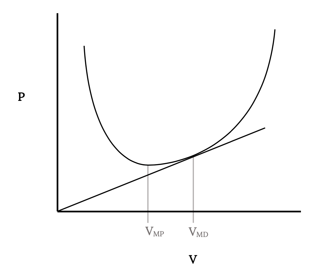
From the above equations it is obvious that, for a given specific fuel consumption and efficiency, the rate of fuel use is a minimum (instantaneous endurance is a maximum) when the power required (DV) is a minimum. It is also obvious that the fuel use per amount of distance traveled is a minimum (instantaneous range is a maximum) when the drag is a minimum.
So we again run into our old friends minimum power required and minimum drag as conditions needed for optimum flight. We already know how to find these graphically from power versus velocity plots as shown below. This graphical determination of minimum power and minimum drag speeds is valid for any drag polar, even if not parabolic.
At this point we should pause and say: “Hey, wait just a minute! It was only a couple of pages back that you said that maximum endurance occurred at minimum drag conditions. Now you say it’s maximum range that I get at minimum drag conditions. Make up your mind, for Pete’s sake!”
The problem is that in one case we are talking about jets and the other, prop aircraft. This means that we must be very careful to see which type of plane we are dealing with before starting any calculations. It is very easy to get into a big rush and get the two cases mixed up (especially in the heat of battle on a test or exam!).
Now, as we did for the jet, we can develop integrals to determine the range or endurance for any flight situation. For endurance we have

and for range

6.5 Approximate Solutions for Range and Endurance for a Prop Aircraft
Once more we will assume “quasi‑level” flight and manipulate the terms in our force balance relations to give
\[D = W\left[\dfrac{D}{L}\right] = W\left[\dfrac{C_D}{C_L}\right]\]
This makes the endurance integral
\[\mathrm{E}=-\int_{W_{1}}^{\mathrm{W} 2} \frac{\eta_{\mathrm{p}}}{\gamma_{\mathrm{p}}} \frac{1}{\mathrm{~V}} \frac{\mathrm{C}_{\mathrm{L}}}{\mathrm{C}_{\mathrm{D}}} \frac{\mathrm{d} \mathrm{W}}{\mathrm{W}}\]
Using the straight and level velocity relation
\[\mathrm{V}=\left[2 \mathrm{~W} /\left(\rho \mathrm{SC}_{\mathrm{L}}\right)\right]^{1 / 2}\]
we get
\[\mathbf{E}=-\int_{\mathbf{W} 1}^{\mathrm{W} 2} \frac{\eta_{\mathrm{p}}}{\gamma_{\mathrm{p}}}[\rho \mathrm{S} / 2]^{1 / 2} \frac{\mathrm{C}_{\mathrm{L}}^{3 / 2}}{\mathrm{C}_{\mathrm{D}}} \frac{\mathrm{dW}}{\mathrm{W}^{3 / 2}}\]
The range integral can be written in a similar fashion as
\[R=-\int_{W_{1}}^{W_{2}} \frac{\eta_{P}}{\gamma_{P}} \frac{C_{L}}{C_{D}} \frac{d W}{W}\]
Now we need to consider the same flight schedules examined in the jet case. Constant angle of attack flight will give constant lift and drag coefficients and constant altitude will give constant density. We will also assume constant specific fuel consumption.
For range we need only to use the constant angle of attack assumption to give a simple integral. The resulting range is
\[R=\frac{\eta_{P}}{\gamma_{P}} \frac{C_{L}}{C_{D}} \ln \left(\frac{W_{1}}{W_{2}}\right), \quad(\text { const } \alpha)\]
For endurance we will consider two cases. The first holds both altitude and angle of attack constant, giving
\[E=-\frac{\eta_{P}}{\gamma_{P}} \sqrt{\frac{\rho S}{2}} \frac{C_{L}^{3 / 2}}{C_{D}} \int_{W_{1}}^{W_{2}} \frac{d W}{W^{3 / 2}}\]
which integrates to
\[E=\frac{\eta_{P}}{\gamma_{P}} \sqrt{2 \rho S} \frac{C_{L}^{3 / 2}}{C_{D}}\left(\frac{1}{\sqrt{W_{2}}}-\frac{1}{\sqrt{W_{1}}}\right),\left(\begin{array}{l}
\text { const } \alpha \\
\text { const } \rho
\end{array}\right)\]
The second case has angle of attack and velocity constant
\[E=-\frac{\eta_{P}}{\gamma_{P}} \frac{1}{V} \frac{C_{L}}{C_{D}} \int_{W_{1}}^{W_{2}} \frac{d W}{W}\]
or
\[E=\frac{\eta_{P}}{\gamma_{P}} \frac{1}{V} \frac{C_{L}}{C_{D}} \ln \left(\frac{W_{1}}{W_{2}}\right), \quad\left(\begin{array}{l}
\text { const } \alpha \\
\text { const } V
\end{array}\right)\]
This is the “drift up” flight schedule.
6.6 Wind Effects
The above range and endurance equations for both jet or prop aircraft were derived assuming no atmospheric winds. The speeds in the equations are the airspeeds, not speeds over the ground. If there is a wind the airspeed is, of course, not equal to the speed over the ground.
Endurance calculations are not altered by the presence of an atmospheric wind. If our concern is how long the aircraft can stay in the air at a given airspeed and altitude and we don’t particularly care if it is making progress over the ground we need not worry about winds. We are doing endurance calculations based only on the aerodynamic behavior of the airplane at a given speed and altitude in a mass of air.
Range is related to speed across the ground rather than the airspeed; thus, if there is a wind our range equation results need to be re-evaluated to account for the wind. The logic of this is simple: a headwind will slow progress over the ground and reduce range while a tailwind will increase range. What is not so obvious is how to correct the calculations to account for this wind. Since our usual concern is to find the maximum range, we will examine the correction for wind effects only for this optimum situation.
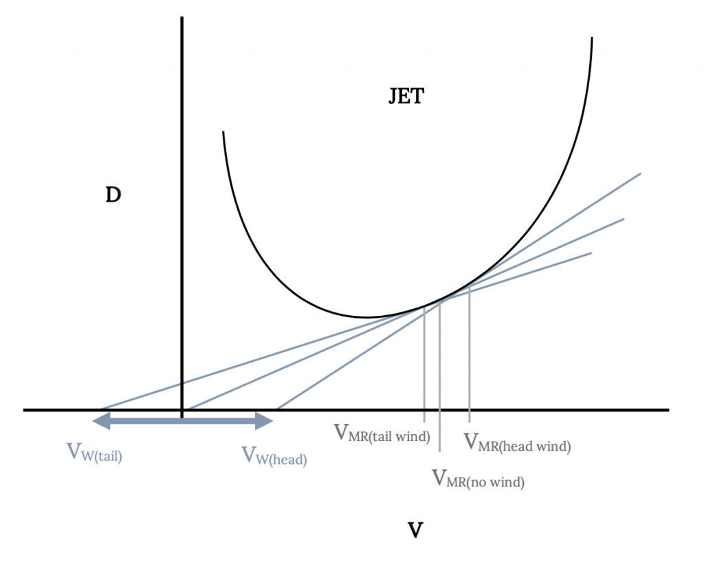
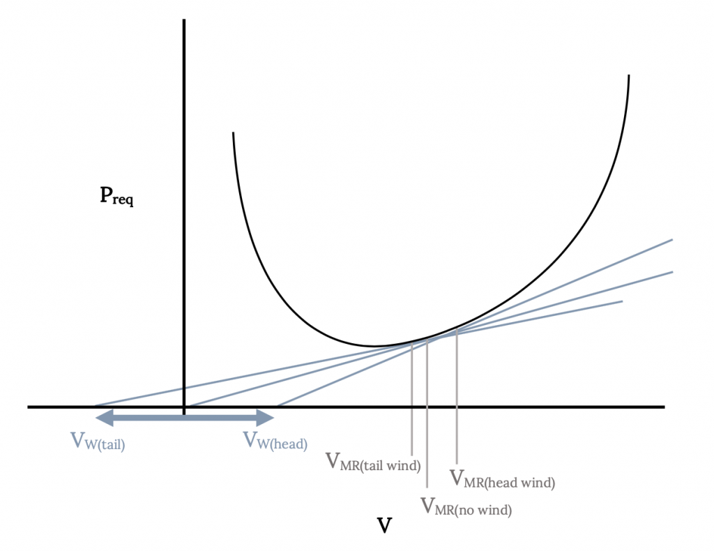
Maximum range for a jet was found to occur when D / V was a minimum while, for a prop, maximum range occurred at minimum drag conditions. The velocities for both cases can be determined graphically by finding the point of tangency for a line drawn from the zero velocity origin on either the drag versus velocity curve in the jet case or the power required versus velocity curve for the prop plane. We can use an extension of this graphical approach to find the speed for best range with either a head wind or a tail wind.
The important first step in determining optimum range in the presence of an atmospheric wind is to find a new airspeed for best range with a wind. This new speed will then be used to calculate a new value of the optimum range. The new value of best range airspeed is found as illustrated in the figures below. The first task is to draw a conventional drag versus velocity (for a jet) or power required versus velocity (for a prop) plot. To this plot is added a new origin, displaced to the left by the value of a tailwind or to the right by the magnitude of the tailwind. A line is then drawn from the displaced origin, tangent to the drag or power curve and the point of tangency locates the new velocity for optimum range with a wind. The magnitude of this new optimum range velocity is read with respect to the original origin (not the displaced origin). This speed is an airspeed, not a ground speed.
This new optimum range velocity is then used to find a new range value from the same equations developed previously. Using the new velocity, new values of lift and drag coefficients are first calculated and these new coefficients and velocity are used to find the optimum range with the wind. To this new range must be added another range which results purely from the aircraft’s time of exposure (endurance) to the wind. This endurance is also found using the newly found optimum range velocity and associated coefficients. The final corrected range for maximum range in a wind is
Rwith wind = RCorrected + VwECorrected for a tailwind
or
Rwith wind = RCorrected – VwECorrected for a headwind
6.7 Let the Buyer Beware
Airplane manufacturers, like those of automobiles and other products, like to do anything they can to make their product look good and sometimes they hope that the buyer doesn’t look too closely at the contradictions in their specifications and advertising. A car may be advertised as having seating for five, an EPA fuel economy rating of 38 mpg, the ability to go 542 miles on a single tank of gas and a top speed of 120 miles per hour. Most of us, however, know not to expect that car to go 542 miles on a single tank of gas while carrying 5 people at a speed of 120 mph! Those who believe it will would also probably be dumb enough to pay sticker price.
What about airplanes? Is this product of an industry which is regulated at every step by the FAA just as subject to contradiction in specifications as a car?
Let’s look at a few simple examples taken from a general aviation Aircraft Fleet Directory of a few years back. A Cessna 150, the most widely used two place aircraft in the country, quotes a range of 815 nautical miles on 32 gallons (210 pounds) of fuel. The plane has an empty weight (no pilot, passenger, baggage or fuel) of 1104 pounds and a maximum gross takeoff weight of 1600 pounds. This means that with the full fuel tanks needed for maximum range there is only a 286 pound allowance for both pilot and passenger, hardly enough for two adults and luggage! This is why one of the favorite questions of flight examiners who are preparing for a private pilot check‑ride in a Cessna 150 involves weight and balance of the aircraft and why sometimes pilots may have to actually pump fuel out of an airplane before takeoff.
A Cessna 172, the most popular four place aircraft in the world, is a little better than the 150 cited above. It has an empty weight of 1387 pounds and to reach its advertised range of 742 miles it has a fuel tank which holds 288 pounds of gas. This gives a total weight for airplane and fuel of 1675 pounds. The maximum gross takeoff weight of the 172 is 2300 pounds, leaving 625 pounds allowance for four passengers and their stuff; an average of 156 pounds each! It is beginning to look like airplanes are designed like those “four-place” cars which have a rear seat about large enough to seat two small poodles!
With another Cessna product, the all around best of their 4 seat line , the Skylane, things are a little better. Its listed empty weight of 1707 pounds, range of 979 nautical miles on 474 pounds of fuel and max gross weight of 2950 pounds leave 769 pounds for pilot, passengers and accessories (192 pounds each). Finally an airplane for real people!
Lest the naive get the idea that this is only a problem for small single engine airplanes, let’s look at one more example, the eight place Learjet 25C. It claims a range of 2472 miles, just the ticket for the rich young business tycoon to fill with seven of her closest friends for a transcontinental weekend jaunt. The listed fuel capacity of 7393 pounds, adds to the quoted “zero fuel” weight of 11,400 pounds to give a 18,793 pound airplane. So how much is left for those 8 passengers? The listed max gross weight of the Learjet 25C is 15,000 pounds! With a full tank of gas the airplane is over its maximum allowable takeoff weight! With a 160 pound pilot and no other passengers or payload this airplane can carry enough fuel for a real range of about 1150 miles, less than half that advertised. Why claim a range of almost 2500 miles? Well, the fuel tanks are big enough to carry the needed fuel. If only the airplane could get off the ground!
Homework 6
1. An aircraft weighs 56,000 pounds and has 900ft2 wing area. Its drag polar equation is given by CD= 0.016 + 0.04CL2. The plane has a turbojet engine with constant thrust at any given altitude as shown below:
Table 6.1: Question 1
| altitude (ft) | 0 | 5000 | 10,000 | 15,000 | 20,000 | 25,000 | 30,000 |
| thrust (lb) | 6420 | 5810 | 5200 | 4590 | 4000 | 3360 | 2700 |
a. Find the minimum thrust required for straight and level flight and the corresponding true airspeeds at sea level and at 30,000 ft.
b. Find the minimum power required and the corresponding true airspeeds at sea level and 30,000 ft.
2. For the aircraft above:
a. plot thrust and drag vs Vefor straight and level flight.
b. plot altitude vs Vemax and Vmax for straight and level flight.
Figure 6.6: Maximum (& Min) Speed for Straight and Level Flight Versus Altitude
c. find the altitude for maximum true airspeed.
d. find the maximum obtainable altitude.
e. compare V at minimum drag from the plot and the calculation.
f. calculate (L/D)max.
References
Figure 6.1: Kindred Grey (2021). “Finding Velocity for Maximum Range .” CC BY 4.0. Adapted from James F. Marchman (2004). CC BY 4.0. Available from https://archive.org/details/6.1-updated
Figure 6.2: Kindred Grey (2021). “Velocities for Minimum Power and Drag.” CC BY 4.0. Adapted from James F. Marchman (2004). CC BY 4.0. Available from https://archive.org/details/6.2-updated
Figure 6.3: Kindred Grey (2021). “Speed for Best Range with Wind (Jet).” CC BY 4.0. Adapted from James F. Marchman (2004). CC BY 4.0. Available from https://archive.org/details/6.3-updated
Figure 6.4: Kindred Grey (2021). “Speed for Best Range with Wind (Prop).” CC BY 4.0. Adapted from James F. Marchman (2004). CC BY 4.0. Available from https://archive.org/details/6.4-updated
Figure 6.5: Kindred Grey (2021). “Thrust and Drag Versus V_e For Straight and Level Flight.” CC BY 4.0. Adapted from James F. Marchman (2004). CC BY 4.0. Available from https://archive.org/details/hw-6-part-1
Figure 6.6: Kindred Grey (2021). “Maximum (& Min) Speed for Straight and Level Flight Versus Altitude.” CC BY 4.0. Adapted from James F. Marchman (2004). CC BY 4.0. Available from https://archive.org/details/hw-6-part-2
- The term “aero-plane” originally referred to a wing, a geometrically planar surface meant to support a vehicle in flight through the air. By 1903 the term had become associated with the entire flying vehicle. By the 1920s the American press and magazines had changed the word to “airplanes”; however, it is still common in Britain to see “aeroplane” used in books and papers. ↵
<!– pb_fixme –><!– pb_fixme –>