
7.7: The Sliding Flow Regime
- Page ID
- 31626

\( \newcommand{\vecs}[1]{\overset { \scriptstyle \rightharpoonup} {\mathbf{#1}} } \)
\( \newcommand{\vecd}[1]{\overset{-\!-\!\rightharpoonup}{\vphantom{a}\smash {#1}}} \)
\( \newcommand{\dsum}{\displaystyle\sum\limits} \)
\( \newcommand{\dint}{\displaystyle\int\limits} \)
\( \newcommand{\dlim}{\displaystyle\lim\limits} \)
\( \newcommand{\id}{\mathrm{id}}\) \( \newcommand{\Span}{\mathrm{span}}\)
( \newcommand{\kernel}{\mathrm{null}\,}\) \( \newcommand{\range}{\mathrm{range}\,}\)
\( \newcommand{\RealPart}{\mathrm{Re}}\) \( \newcommand{\ImaginaryPart}{\mathrm{Im}}\)
\( \newcommand{\Argument}{\mathrm{Arg}}\) \( \newcommand{\norm}[1]{\| #1 \|}\)
\( \newcommand{\inner}[2]{\langle #1, #2 \rangle}\)
\( \newcommand{\Span}{\mathrm{span}}\)
\( \newcommand{\id}{\mathrm{id}}\)
\( \newcommand{\Span}{\mathrm{span}}\)
\( \newcommand{\kernel}{\mathrm{null}\,}\)
\( \newcommand{\range}{\mathrm{range}\,}\)
\( \newcommand{\RealPart}{\mathrm{Re}}\)
\( \newcommand{\ImaginaryPart}{\mathrm{Im}}\)
\( \newcommand{\Argument}{\mathrm{Arg}}\)
\( \newcommand{\norm}[1]{\| #1 \|}\)
\( \newcommand{\inner}[2]{\langle #1, #2 \rangle}\)
\( \newcommand{\Span}{\mathrm{span}}\) \( \newcommand{\AA}{\unicode[.8,0]{x212B}}\)
\( \newcommand{\vectorA}[1]{\vec{#1}} % arrow\)
\( \newcommand{\vectorAt}[1]{\vec{\text{#1}}} % arrow\)
\( \newcommand{\vectorB}[1]{\overset { \scriptstyle \rightharpoonup} {\mathbf{#1}} } \)
\( \newcommand{\vectorC}[1]{\textbf{#1}} \)
\( \newcommand{\vectorD}[1]{\overrightarrow{#1}} \)
\( \newcommand{\vectorDt}[1]{\overrightarrow{\text{#1}}} \)
\( \newcommand{\vectE}[1]{\overset{-\!-\!\rightharpoonup}{\vphantom{a}\smash{\mathbf {#1}}}} \)
\( \newcommand{\vecs}[1]{\overset { \scriptstyle \rightharpoonup} {\mathbf{#1}} } \)
\(\newcommand{\longvect}{\overrightarrow}\)
\( \newcommand{\vecd}[1]{\overset{-\!-\!\rightharpoonup}{\vphantom{a}\smash {#1}}} \)
\(\newcommand{\avec}{\mathbf a}\) \(\newcommand{\bvec}{\mathbf b}\) \(\newcommand{\cvec}{\mathbf c}\) \(\newcommand{\dvec}{\mathbf d}\) \(\newcommand{\dtil}{\widetilde{\mathbf d}}\) \(\newcommand{\evec}{\mathbf e}\) \(\newcommand{\fvec}{\mathbf f}\) \(\newcommand{\nvec}{\mathbf n}\) \(\newcommand{\pvec}{\mathbf p}\) \(\newcommand{\qvec}{\mathbf q}\) \(\newcommand{\svec}{\mathbf s}\) \(\newcommand{\tvec}{\mathbf t}\) \(\newcommand{\uvec}{\mathbf u}\) \(\newcommand{\vvec}{\mathbf v}\) \(\newcommand{\wvec}{\mathbf w}\) \(\newcommand{\xvec}{\mathbf x}\) \(\newcommand{\yvec}{\mathbf y}\) \(\newcommand{\zvec}{\mathbf z}\) \(\newcommand{\rvec}{\mathbf r}\) \(\newcommand{\mvec}{\mathbf m}\) \(\newcommand{\zerovec}{\mathbf 0}\) \(\newcommand{\onevec}{\mathbf 1}\) \(\newcommand{\real}{\mathbb R}\) \(\newcommand{\twovec}[2]{\left[\begin{array}{r}#1 \\ #2 \end{array}\right]}\) \(\newcommand{\ctwovec}[2]{\left[\begin{array}{c}#1 \\ #2 \end{array}\right]}\) \(\newcommand{\threevec}[3]{\left[\begin{array}{r}#1 \\ #2 \\ #3 \end{array}\right]}\) \(\newcommand{\cthreevec}[3]{\left[\begin{array}{c}#1 \\ #2 \\ #3 \end{array}\right]}\) \(\newcommand{\fourvec}[4]{\left[\begin{array}{r}#1 \\ #2 \\ #3 \\ #4 \end{array}\right]}\) \(\newcommand{\cfourvec}[4]{\left[\begin{array}{c}#1 \\ #2 \\ #3 \\ #4 \end{array}\right]}\) \(\newcommand{\fivevec}[5]{\left[\begin{array}{r}#1 \\ #2 \\ #3 \\ #4 \\ #5 \\ \end{array}\right]}\) \(\newcommand{\cfivevec}[5]{\left[\begin{array}{c}#1 \\ #2 \\ #3 \\ #4 \\ #5 \\ \end{array}\right]}\) \(\newcommand{\mattwo}[4]{\left[\begin{array}{rr}#1 \amp #2 \\ #3 \amp #4 \\ \end{array}\right]}\) \(\newcommand{\laspan}[1]{\text{Span}\{#1\}}\) \(\newcommand{\bcal}{\cal B}\) \(\newcommand{\ccal}{\cal C}\) \(\newcommand{\scal}{\cal S}\) \(\newcommand{\wcal}{\cal W}\) \(\newcommand{\ecal}{\cal E}\) \(\newcommand{\coords}[2]{\left\{#1\right\}_{#2}}\) \(\newcommand{\gray}[1]{\color{gray}{#1}}\) \(\newcommand{\lgray}[1]{\color{lightgray}{#1}}\) \(\newcommand{\rank}{\operatorname{rank}}\) \(\newcommand{\row}{\text{Row}}\) \(\newcommand{\col}{\text{Col}}\) \(\renewcommand{\row}{\text{Row}}\) \(\newcommand{\nul}{\text{Nul}}\) \(\newcommand{\var}{\text{Var}}\) \(\newcommand{\corr}{\text{corr}}\) \(\newcommand{\len}[1]{\left|#1\right|}\) \(\newcommand{\bbar}{\overline{\bvec}}\) \(\newcommand{\bhat}{\widehat{\bvec}}\) \(\newcommand{\bperp}{\bvec^\perp}\) \(\newcommand{\xhat}{\widehat{\xvec}}\) \(\newcommand{\vhat}{\widehat{\vvec}}\) \(\newcommand{\uhat}{\widehat{\uvec}}\) \(\newcommand{\what}{\widehat{\wvec}}\) \(\newcommand{\Sighat}{\widehat{\Sigma}}\) \(\newcommand{\lt}{<}\) \(\newcommand{\gt}{>}\) \(\newcommand{\amp}{&}\) \(\definecolor{fillinmathshade}{gray}{0.9}\)7.7.1 Introduction
Vlasak et al. (2012) and (2014) investigated the transport of coarse particles in a Dp=0.1 m pipe in the Institute of Hydrodynamics in Prague. The particles had a d50=11.0-11.7 mm diameter and were transported with line speeds in the range of 1.5 m/s to 5.5 m/s. The density of the particles is 2.787 ton/m3 and the carrier liquid was water. Concentrations in the range of 3% to 15% were used. So, the particles had a diameter of about 10-11% of the pipe diameter.
In the horizontal pipe section the flow was significantly stratified. For low line speeds the individual particles were sliding and rolling over the bottom of the pipe. Increasing the line speed resulted in ripples and dunes. In the lower line speed range the sliding bed layer was combined with saltation on top of the bed and dunes appearing and disappearing. With increasing line speed the thickness of the sliding bed decreased and particle saltation became the dominant mode of particle movement. However, most particles remained in contact with the pipe wall. The pressure drops were mainly produced by mechanical friction between the particles and the pipe wall, also resulting in relatively high slip ratio values. The transport was dominated by particle-particle interactions and particle-wall interactions. The horizontal particle velocities increased with the vertical distance from the pipe bottom. Saltating (free) particles had a much higher horizontal velocity compared with the particles in the bed.
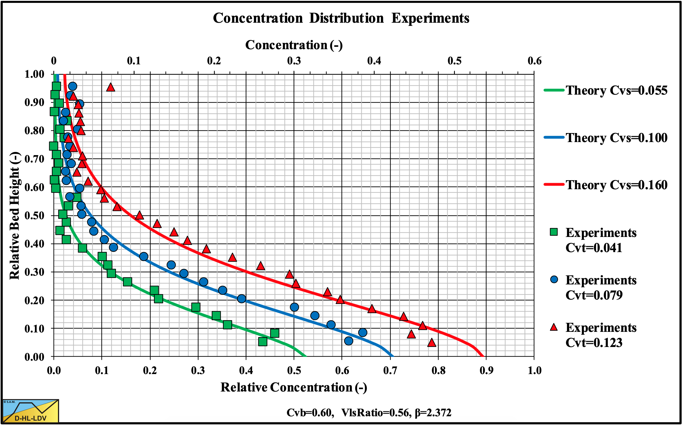
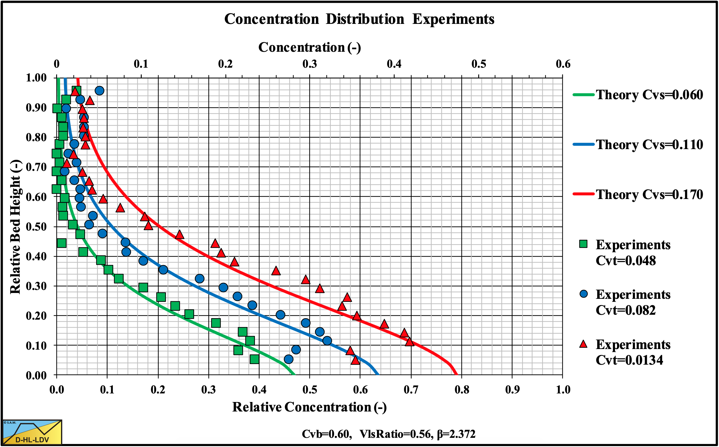
The concentration distribution is important to understand the internal structure of the mixture flow. At low line speeds (Figure 7.7-9) the local concentration tends to approach zero at the upper portion of the pipe. This region increased with decreasing concentration and occupied 30%-50% of the pipe. A nearly linear concentration profile was observed in the lower part of the pipe, increasing from a bottom concentration at the bottom of the pipe to almost zero at a height of 50%-70% of the pipe. The bottom concentration decreased with a decreasing cross sectional averaged concentration. Very dense sand or gravel has a concentration up to 66%. Very loose sand or gravel a concentration of about 50%. Below 50% the particles do not rest on top of each other, however in a fast- flowing sliding bed this is possible because of the kinetic particle-particle interactions. Moderate line speeds (Figure 7.7-10) showed the same behavior, but with smaller bottom concentrations. At high line speeds (Figure 7.7-11) the bottom concentrations decreased further, but with the same shape of the concentration profile. In general, the particles tend to occupy the bottom part of the pipe and the concentration profile is symmetrical to the vertical plane of symmetry. The higher concentrations shown at the top of the pipe were detected as errors due to the effect of the pipe material on gamma-ray absorption.
According to the DHLLDV Framework of Miedema (June 2016) the Limit Deposit Velocity (LDV) of the particles used by Vlasak et al. (2012) and (2014) has a value around 3 m/s. For small particles, this LDV is the velocity above which no stationary or sliding bed exists. It is the question however whether for such large particles an LDV still exists since the particles continue to occupy the bottom part of the pipe even at high line speeds. Maybe at low concentrations this may be the case, but at high concentrations there is not enough turbulent energy to completely remove the bed. It seems also at high line speeds there is still a sort of bed, but with decreased concentration as the line speed increases.
Apparently very coarse particles do not follow the heterogeneous and homogeneous flow regimes at high line speeds as has been described by Miedema (June 2016), but follow a different behavior, which is named the sliding flow regime. In the sliding flow regime, the hydraulic gradient is dominated by sliding and/or rolling friction instead of collisions as in the heterogeneous regime. As long as the bed has a high concentration preventing the particles to start rolling, the normal sliding friction coefficient as used in the sliding bed regime can be applied. However, if the bed concentration reduces below 50%, giving particles more freedom to roll, the observed sliding friction coefficient may reduce because the rolling friction coefficient is always smaller than the sliding friction coefficient.
7.7.2 Literature & Theory
For fine and medium sized particles there is a transition from a sliding bed to heterogeneous transport at a certain line speed. However for large particles the turbulence is not capable of lifting the particles enough resulting in a sort of sliding bed behavior above this transition line speed. One reason for this is that the largest eddies are not large enough with respect to the size of the particles. Sellgren & Wilson (2007) use the criterion d/Dp>0.015 for this to occur. Zandi & Govatos (1967) use a factor N<40 as a criterion, with:
\[\ \mathrm{N}=\frac{\mathrm{v}_{\mathrm{l} \mathrm{s}}^{2} \cdot \sqrt{\mathrm{C}_{\mathrm{x}}}}{\mathrm{g} \cdot \mathrm{R}_{\mathrm{s} \mathrm{d}} \cdot \mathrm{D}_{\mathrm{p}} \cdot \mathrm{C}_{\mathrm{v} \mathrm{t}}}\]
At the Limit Deposit Velocity vls,ldv this equation can be simplified for coarse particles by using:
\[\ \mathrm{F}_{\mathrm{L}}=\frac{\mathrm{v}_{\mathrm{l s}, \mathrm{ld} \mathrm{v}}}{\sqrt{\mathrm{2 \cdot g} \cdot \mathrm{D}_{\mathrm{p}} \cdot \mathrm{R}_{\mathrm{s d}}}} \approx 1.34\text{ and }\sqrt{\mathrm{C}_{\mathrm{x}}} \approx 0.6\text{ for coarse sand}\]
Giving:
\[\ \mathrm{N}=\frac{\mathrm{v}_{\mathrm{l} \mathrm{s}}^{2} \cdot \sqrt{\mathrm{C}_{\mathrm{x}}}}{\mathrm{g} \cdot \mathrm{R}_{\mathrm{s d}} \cdot \mathrm{D}_{\mathrm{p}} \cdot \mathrm{C}_{\mathrm{v t}}}=\left(\frac{\mathrm{v}_{\mathrm{l} \mathrm{s}}^{2}}{\mathrm{2} \cdot \mathrm{g} \cdot \mathrm{R}_{\mathrm{s d}} \cdot \mathrm{D}_{\mathrm{p}}}\right) \cdot \frac{\mathrm{2} \cdot \sqrt{\mathrm{C}_{\mathrm{x}}}}{\mathrm{C}_{\mathrm{v t}}}=\mathrm{1 . 3 4}^{2} \cdot \frac{\mathrm{2} \cdot \mathrm{0.6}}{\mathrm{C}_{\mathrm{v t}}}=\frac{\mathrm{2.3 7}}{\mathrm{C}_{\mathrm{v t}}}\]
This gives N=2.37/Cvt<40 or Cvt>0.059 for sliding flow to occur. This criterion apparently is based on the thickness of sheet flow. If the bed is so thin that the whole bed becomes sheet flow, there will not be sliding flow, but more heterogeneous behavior. The values used in both criteria are a first estimate based on literature and may be changed in the future.
A pragmatic approach to determine the relative excess hydraulic gradient in the sliding flow regime is to use a weighted average between the heterogeneous regime and the sliding bed regime. First the factor between particle size and pipe diameter is determined:
| \[\ \mathrm{f}=\frac{4}{3}-\frac{1}{3} \cdot \frac{\mathrm{d}}{\mathrm{r}_{\mathrm{d} / \mathrm{D p}} \cdot \mathrm{D}_{\mathrm{p}}} \quad\text{ with: }\mathrm{0} \leq \mathrm{f} \leq \mathrm{1}\] |
Secondly the weighted average hydraulic gradient or relative excess hydraulic gradient is determined:
|
\[ \begin{array}{left}\mathrm{i}_{\mathrm{m}, \mathrm{S F}}=\mathrm{i}_{\mathrm{m}, \mathrm{H} \mathrm{e H o}} \cdot \mathrm{f}+\mathrm{i}_{\mathrm{m}, \mathrm{S B}} \cdot(\mathrm{1}-\mathrm{f}) \\ \text{or}\\ \mathrm{E}_{\mathrm{r h g}, \mathrm{S F}}=\mathrm{E}_{\mathrm{r h g}, \mathrm{H e H o}} \cdot \mathrm{f}+\mu_{\mathrm{s f}} \cdot(\mathrm{1 - f})\end{array}\] |
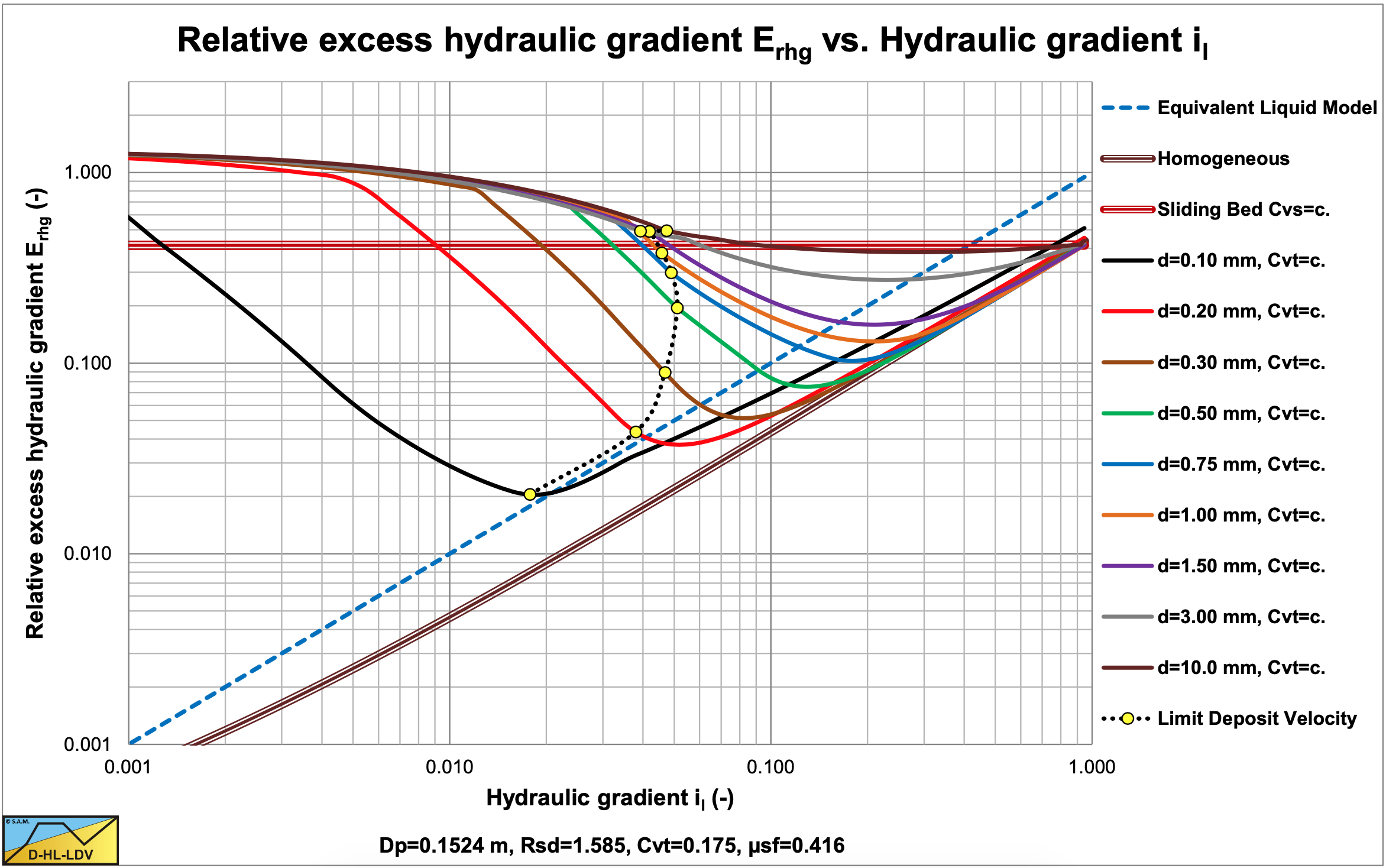
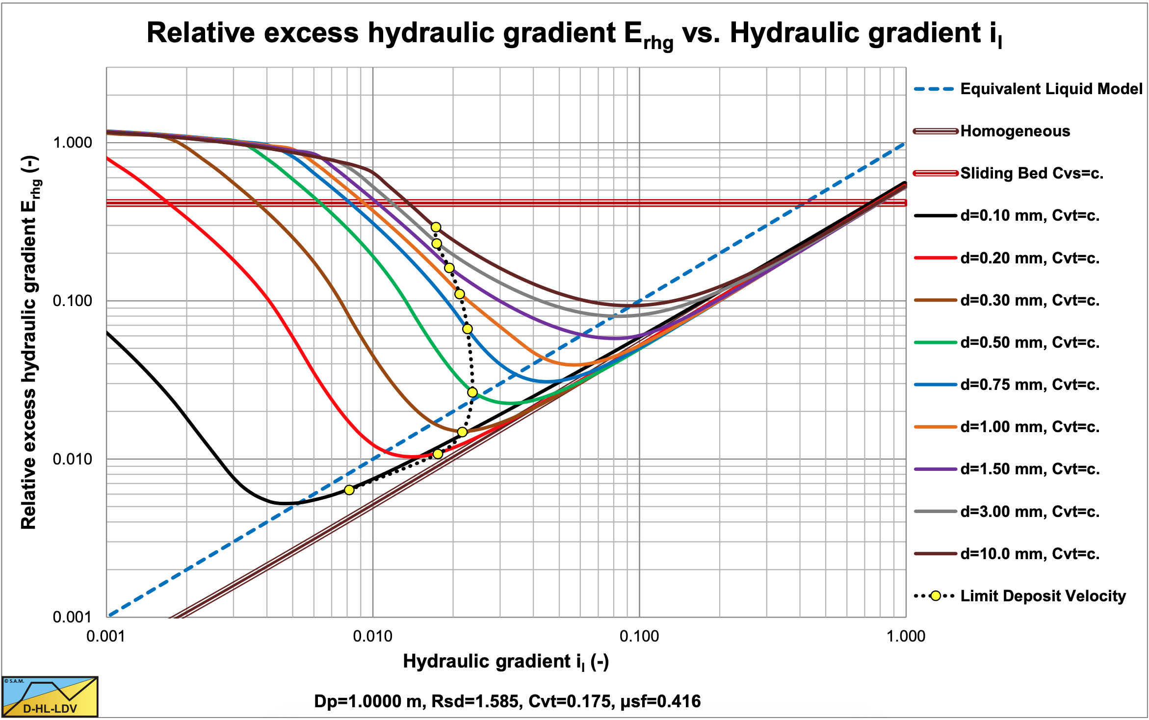
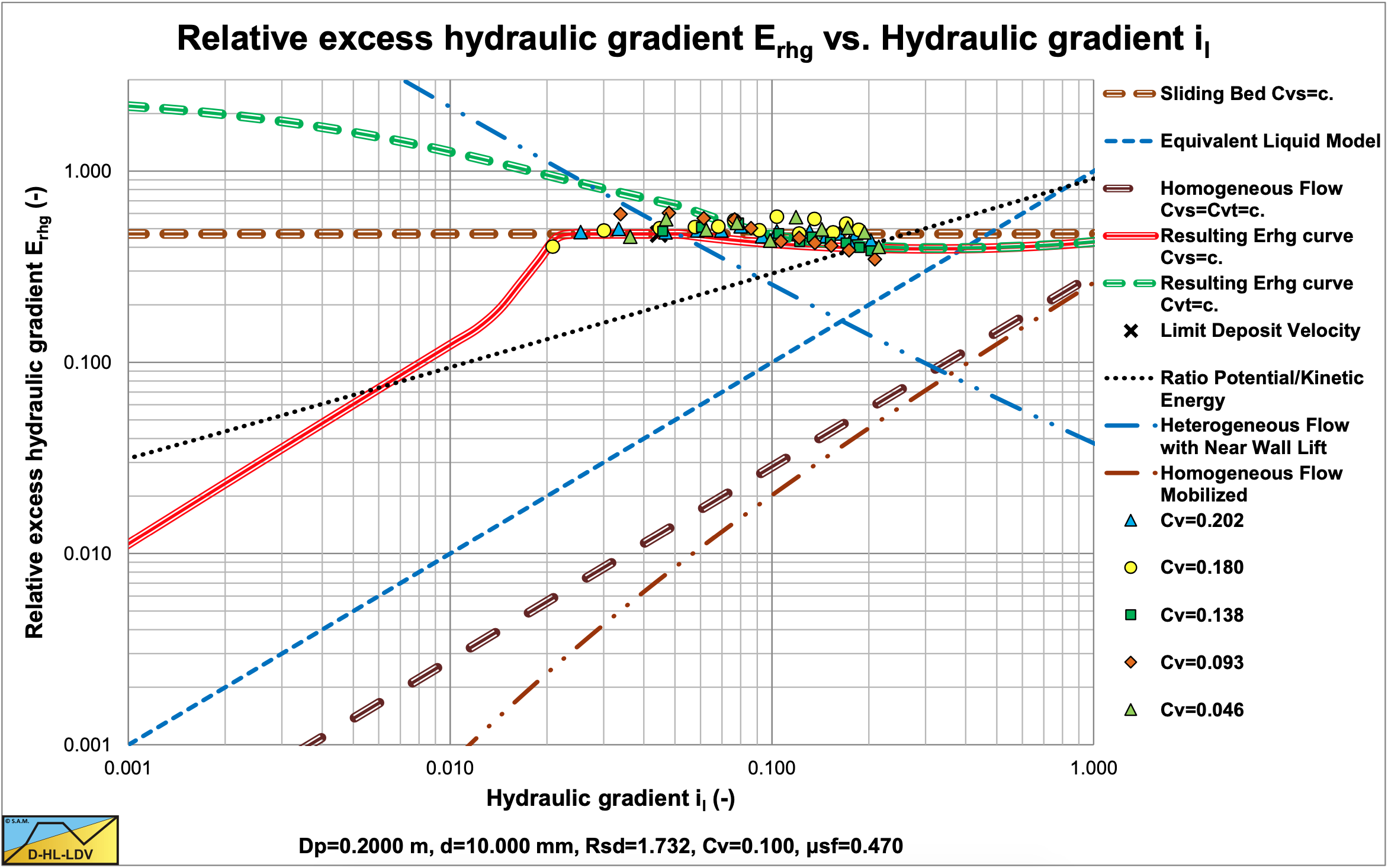
Figure 7.7-1 and Figure 7.7-2 show the relative excess hydraulic gradient of 9 particle diameters for a constant delivered volumetric concentration of 17.5%. The graphs also show the horizontal sliding bed curve for constant spatial volumetric concentration, the ELM curve and the homogeneous curve as a reference system. The LDV points for each particle diameter are also shown.
Figure 7.7-1 shows that large particles in a Dp=0.1524 m pipe have a much less steep curve than the smaller particles due to sliding flow. Sliding flow starts with particles of about d=2.3 mm. Figure 7.7-2 shows that this does not occur in a large Dp=1 m pipe. Here sliding flow starts with particles of about d=15 mm, which are not in the graph.
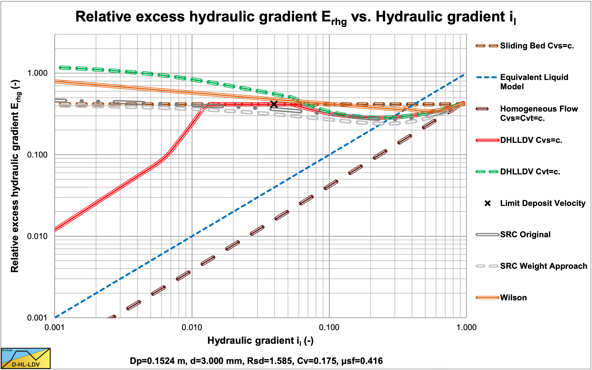
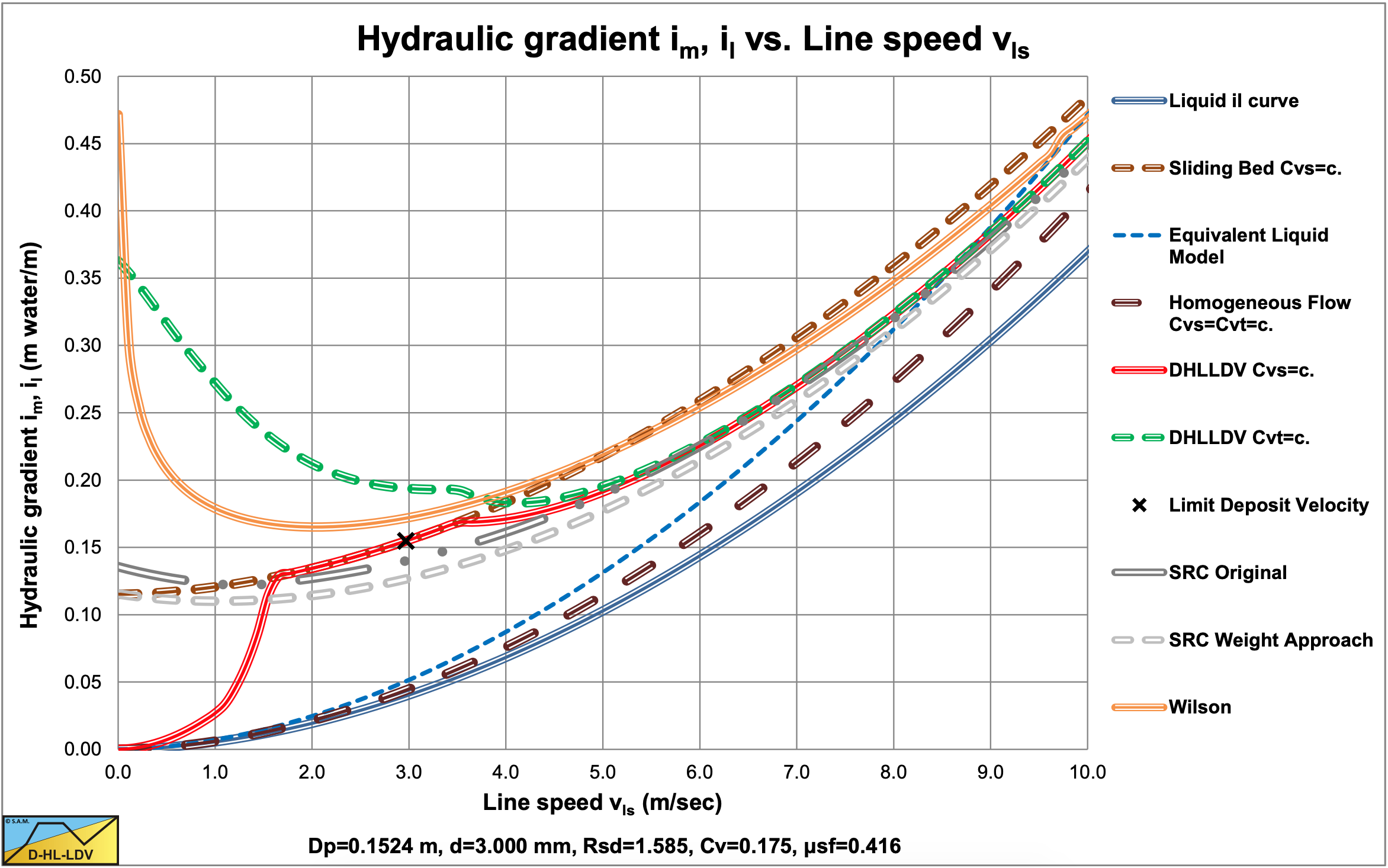
The resulting curves match very well with the SRC model in the range of operational line speeds. Figure 7.7-3 and Figure 7.7-4 show this for a d=3 mm particle in a Dp=0.1524 m (6 inch) pipe.. The SRC model used here is a simplified model as described in chapter 6. The relative hydraulic excess gradient seems to differ, but in the hydraulic gradient graph it is clear that there is not much difference in the range of line speeds of 4-6 m/sec. Both the SRC model and the DHLLDV Framework are based on constant spatial volumetric concentration. The Wilson curve gives a higher curve, but the Wilson model is based on a constant delivered volumetric concentration.
7.7.3 The Concentration Distribution
In the case of Sliding Flow, the bottom concentration decreases with increasing line speed and with decreasing spatial concentration. The bottom concentration can be determined with the following equation, where the bottom concentration can never be larger than the maximum bed concentration Cvb and never smaller than the spatial concentration Cvs. The Limit of Stationary Deposit Velocity (LSDV) has to be determined at a concentration of 17.5%, because the equation is calibrated for Cvs=0.175.
| \[\ \mathrm{C}_{\mathrm{v B}}=\mathrm{3.1} \cdot \mathrm{C}_{\mathrm{v b}} \cdot\left(\frac{\mathrm{v}_{\mathrm{l} \mathrm{s}, \mathrm{l} \mathrm{s} \mathrm{d v}}}{\mathrm{v}_{\mathrm{l s}}}\right)^{0.4} \cdot\left(\frac{\mathrm{C}_{\mathrm{v s}}}{\mathrm{C}_{\mathrm{v b}}}\right)^{0.5} \cdot \mathrm{v}_{\mathrm{t}}^{1/6} \cdot \mathrm{e}^{\mathrm{D}_{\mathrm{p}}} \quad \text{with: } \mathrm{1. 1} \cdot \mathrm{C}_{\mathrm{v s}} \leq \mathrm{C}_{\mathrm{v} \mathrm{B}} \leq \mathrm{C}_{\mathrm{v} \mathrm{b}}\] |
To determine the concentration distribution, the procedure outlined in chapter 7.10 should be followed with a line speed to Limit Deposit Velocity ratio of 1 and a bottom/bed concentration as determined with the above equation. Physically this means that a sliding bed will transit to sliding flow by increasing the porosity between the particles with increasing line speed. The Limit Deposit Velocity has no physical meaning in the Sliding Flow Regime.
The concentration distribution is now:
| \[\ \begin{array}{left} \mathrm{C}_{\mathrm{vs}}(\mathrm{f})=\mathrm{C}_{\mathrm{vB}} \cdot \mathrm{e}^{-\frac{\alpha_{\mathrm{sm}} }{\mathrm{C}_{\mathrm{vr}}}\cdot \mathrm{f}} \quad\text{ with: }\mathrm{C}_{\mathrm{vr}}=\frac{\mathrm{C}_{\mathrm{vs}}}{\mathrm{C}_{\mathrm{vB}}}\\ \alpha_{\mathrm{sm}}=0.9847+0.304 \cdot \mathrm{C}_{\mathrm{vr}}-1.196 \cdot \mathrm{C}_{\mathrm{vr}}^{2}-0.5564 \cdot \mathrm{C}_{\mathrm{vr}}^{3}+0.47 \cdot \mathrm{C}_{\mathrm{vr}}^{4}\end{array}\] |
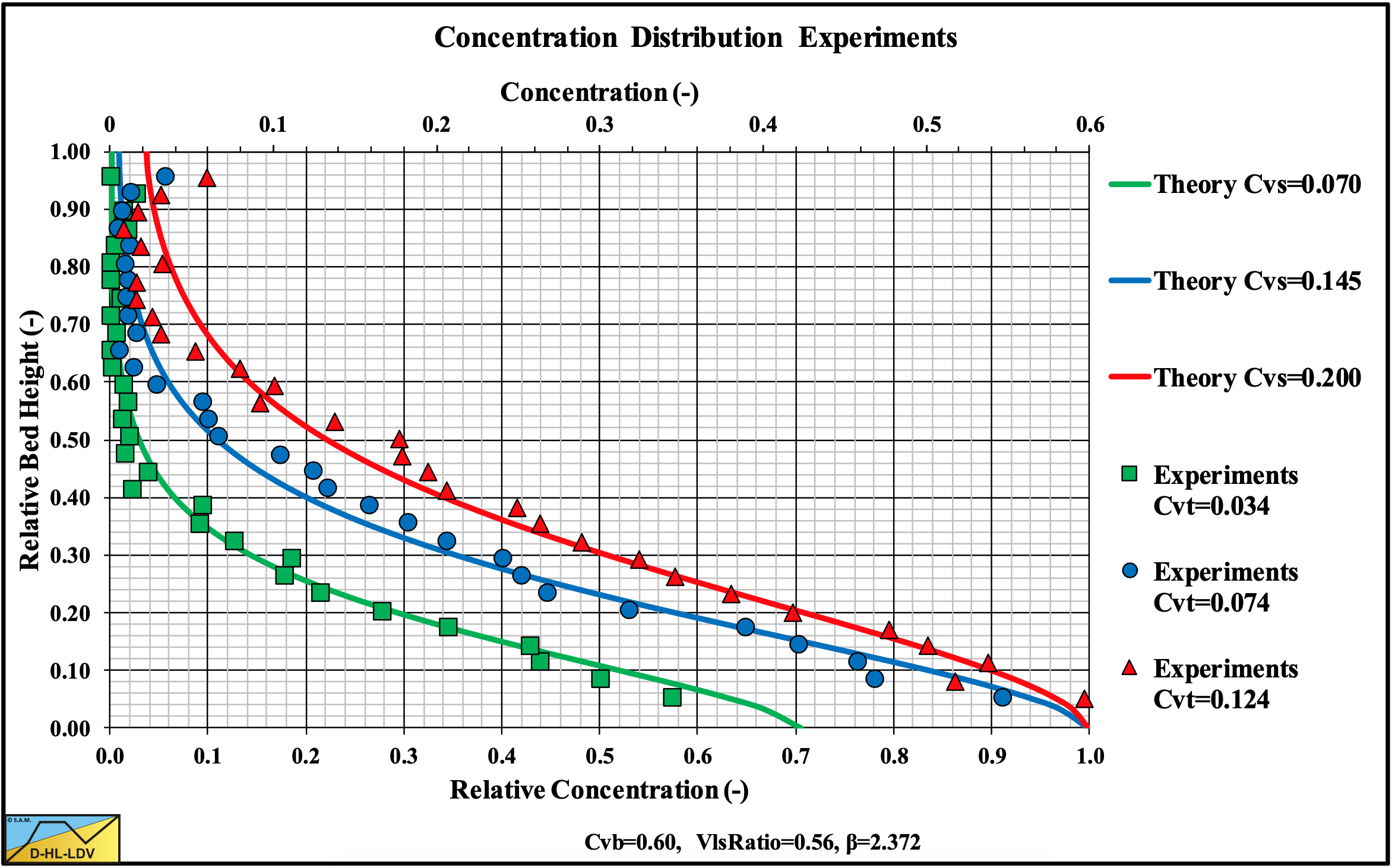
Figure 7.7-9, Figure 7.7-10 and Figure 7.7-11 show experimental results of Vlasak et al. (2014) in a Dp=0.1 m pipe and d=11 mm particles at 3 different line speeds. The d/Dp ratio equals 0.11, so this is certainly in the Sliding Flow regime. The experiments show a decreasing bottom concentration with increasing line speed and a decreasing bottom concentration with decreasing spatial concentration according to the above equation. The volumetric concentrations used to simulate the measured concentration profiles are higher than the volumetric concentrations mentioned by Vlasak et al. (2014). Most probably Vlasak et al. (2014) measured delivered concentrations, while here spatial concentrations should be used. It should be mentioned that the experiments show some small concentration at the top of the pipe, which is not always predicted. The predictions and the experimental data however match well. These experimental concentration profiles required a factor 2 in the hindered settling power instead of the default value of 4.
7.7.4 Verification & Validation
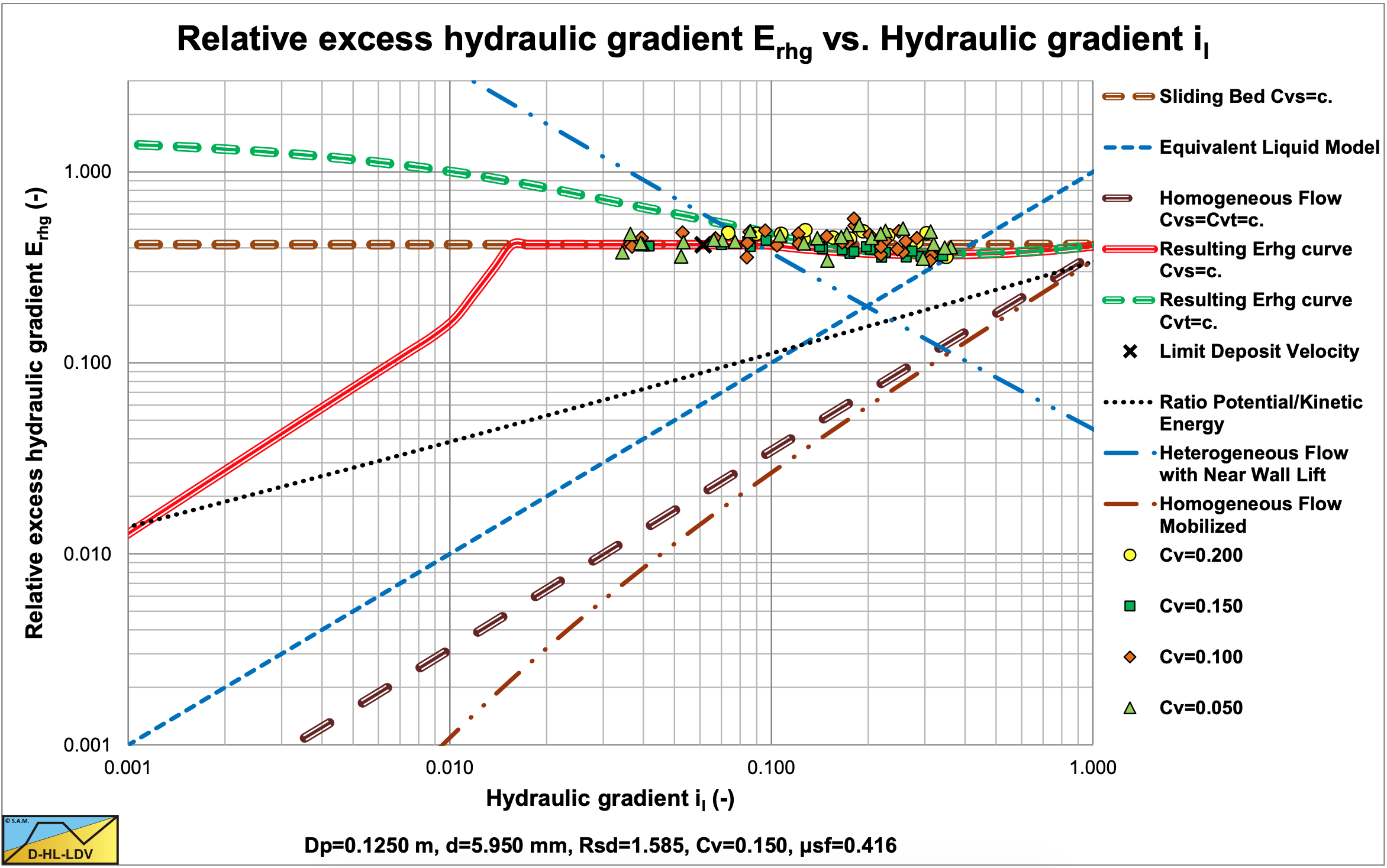
Figure 7.7-5 and Figure 7.7-6 show sliding flow behavior for two types of gravel, with d=6 mm and d=10 mm and constant spatial volumetric concentrations. At higher line speeds or liquid hydraulic gradients the relative excess hydraulic gradient of the DHLLDV Framework tends to decrease slightly. This occurs when the liquid hydraulic gradient is close to the intersection point between the sliding bed/sliding flow curve and the ELM curve. In this region however the line speeds are so high that there are hardly any experimental data available. The data here is obtained from Boothroyde et al. (1979) and Wiedenroth (1967).
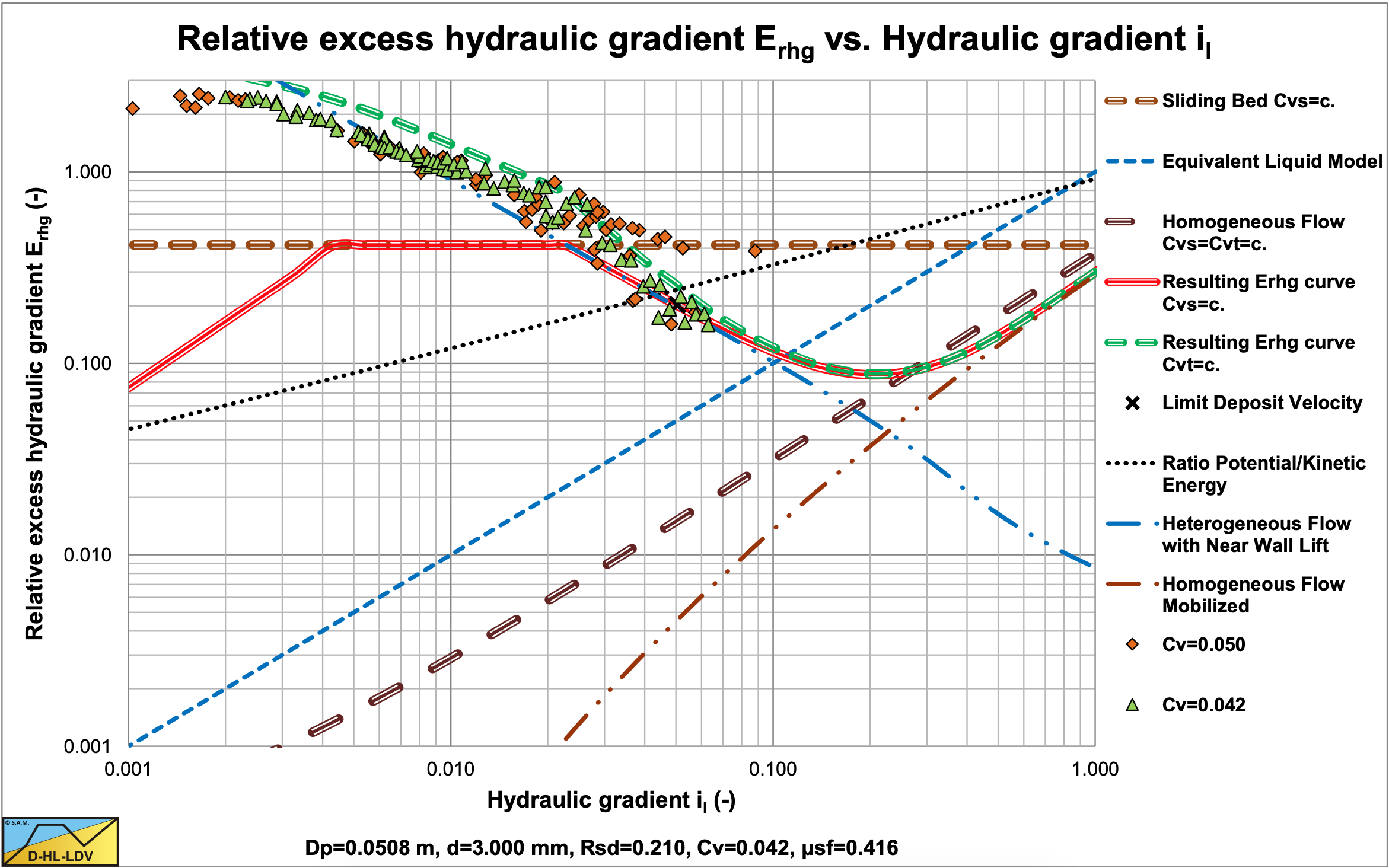
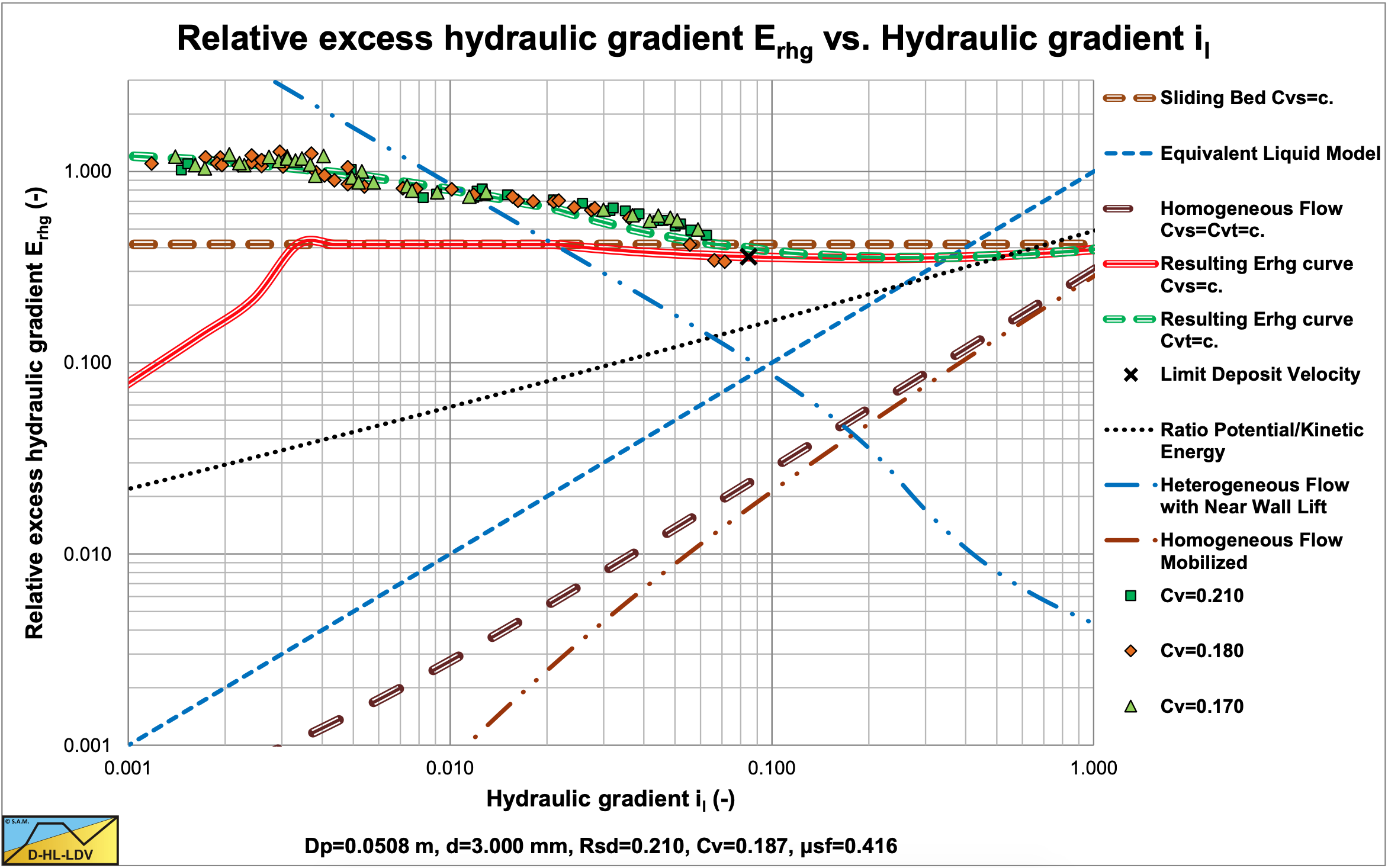
Figure 7.7-7 and Figure 7.7-8 show heterogeneous behavior at very low concentrations and sliding flow behavior at higher concentrations. These experiments by Doron & Barnea (1993) were carried out with delivered volumetric concentration measurements. They clearly show that at very low concentrations there is still heterogeneous behavior, while the higher concentrations show sliding flow behavior.
The weighted average approach seems to give good results. Still the criterion for sliding flow, d>0.015·Dp, is too simple and requires more research, which will be explained in the next chapter.
For the concentration distribution, the bottom/bed concentration has to be determined first. Secondly the concentration profile can be determined based on a line speed to Limit Deposit Velocity ratio of 1.
In the sliding flow regime, the LDV doesn’t really have a physical meaning. At high line speeds the bed continues to show sliding friction behavior, but the porosity of the bed increases with increasing line speed.
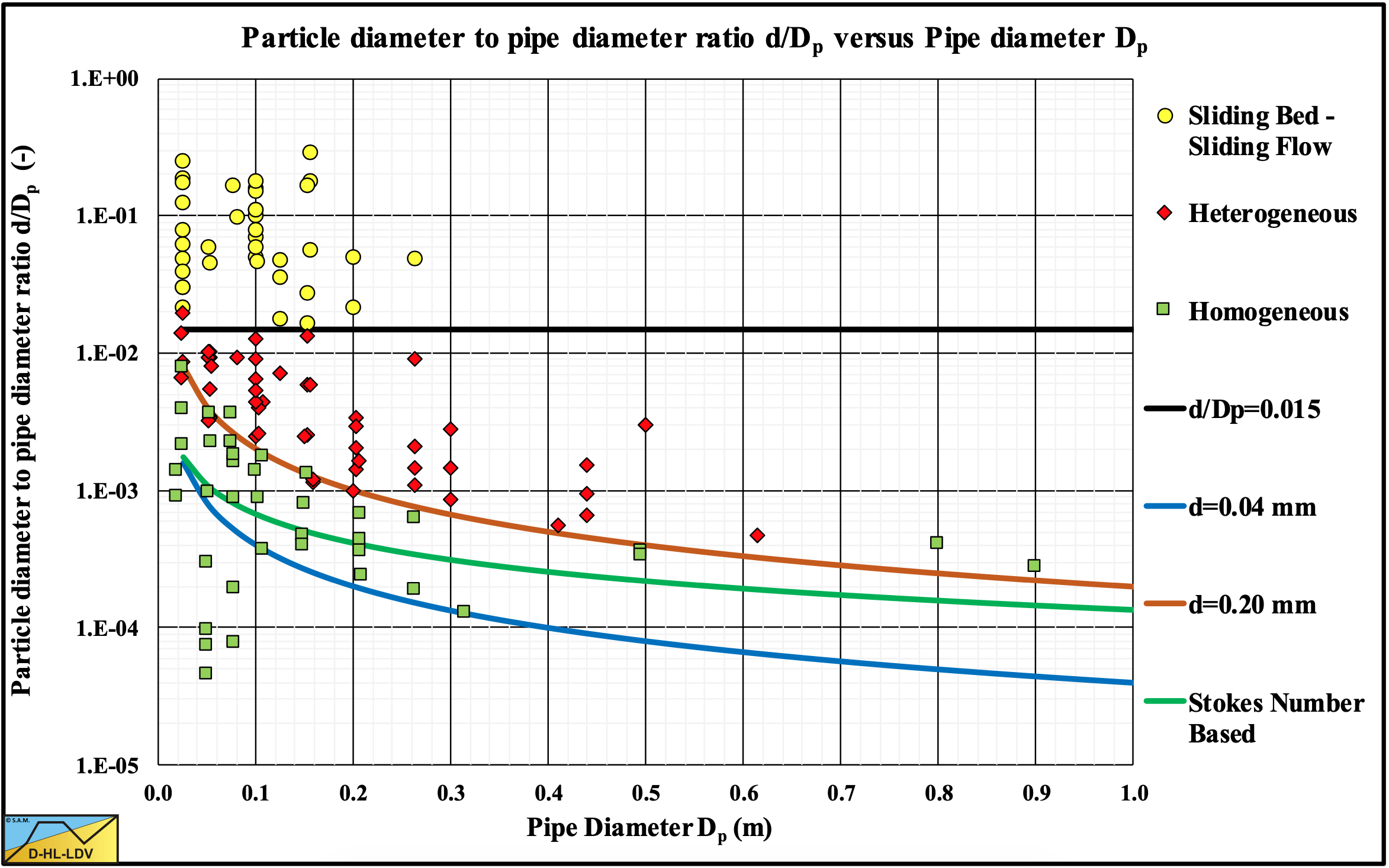
Figure 7.7-12 shows observed heterogeneous and sliding flow (fully stratified) behavior. Heterogeneous behavior means that the heterogeneous curve is followed. Sliding Flow behavior means that the sliding friction curve is followed. The transition between the two flow regimes is close to 0.015 as mentioned by Sellgren & Wilson (2007). However, only experiments in small diameter pipes were found for fully stratified flow. Some experiments close to the 0.015 ratio show transition behavior. The hydraulic gradient curves lie between the heterogeneous and sliding flow curves. Most experiments were carried out with natural particles. Some experiments were carried out with glass and aluminum beads. Since the latter experiments had particles far above the 0.015 ratio, a difference between natural particles and beads could not be distinguished. Also the influence of the volumetric concentration could not be determined, since most experiments were carried out at medium relative volumetric concentrations.
7.7.5 The Particle Diameter to Pipe Diameter Ratio
The particle diameter to pipe diameter ratio, d>0.015·Dp, is to simple. Also, no physical background has been found. So here an attempt is described to find a more fundamental background. The question is, does this ratio only depend on the diameter ratio, or are other parameters like the relative submerged density or the viscosity also involved.
The Sliding Flow Regime is described as a high concentrated flow of particles at the bottom of the pipe, behaving like a sliding bed, but with a lower concentration compared to the bed concentration. The top of this sliding flow may show sheet flow, similar to the sliding bed behavior. Sliding flow means that there is no or hardly any suspension above the sliding flow, the low concentrated bed. This implies that there is an equilibrium of deposition and suspension at the top of the sliding flow layer. The amount of particles being suspended are equal to the amount of particles depositioning. Particles being suspended is related to the bed shear stress or the Shields Number (dimensionless bed shear stress). Particles depositioning (settling) is related to the terminal settling velocity. Since sliding flow means, hardly any suspension above the bed, hindered settling does not have to be taken into account. Since the flow results in sliding friction (sliding bed behavior), an indication of the bed shear stress is available. So the criterion for the particle diameter to pipe diameter is:
\[\ \mathrm{v}_{\mathrm{t}}=\alpha_{\mathrm{s}} \cdot \mathrm{u}_{*}\]
The terminal settling velocity is equal to the so called friction velocity. This is often used as a criterion for suspension vs. no suspension (see also Chapter 5 and Chapter 7.8). This criterion can be translated in terms of the Shields parameter by:
\[\ \mathrm{v}_{\mathrm{t}}=\sqrt{\frac{\mathrm{4 \cdot g \cdot R}_{\mathrm{s d}} \cdot \mathrm{d \cdot \Psi}}{\mathrm{3} \cdot \mathrm{C}_{\mathrm{D}}}}=\alpha_{\mathrm{s}} \cdot \mathrm{u}_{*}\]
Giving:
\[\ \theta=\frac{\mathrm{u}_{*}^{2}}{\mathrm{g} \cdot \mathrm{R}_{\mathrm{s} \mathrm{d}} \cdot \mathrm{d}}=\frac{\mathrm{1}}{\alpha_{\mathrm{s}}^{2}} \cdot \frac{\mathrm{4} \cdot \Psi}{\mathrm{3} \cdot \mathrm{C}_{\mathrm{D}}}\]
For spheres this gives a Shields parameter of 3 and for real sand particles about 1, with αs=1.
For the derivation, first the equilibrium of forces on the layer of liquid above the sliding flow is derived, in order to have an expression for the pressure gradient.
\[\ \tau_{1} \cdot \mathrm{D}_{\mathrm{p}} \cdot(\pi-\beta) \cdot \Delta \mathrm{L}+\tau_{12} \cdot \mathrm{D}_{\mathrm{p}} \cdot \sin (\beta) \cdot \Delta \mathrm{L}=\Delta \mathrm{p} \cdot \mathrm{A}_{\mathrm{p}} \cdot\left(1-\mathrm{C}_{\mathrm{v r}}\right)\]
The bed shear stress equals the carrier liquid density times the friction velocity squared. Now assume the pipe wall shear stress is a factor times the bed shear stress, this gives:
\[\ \alpha_{\tau} \cdot \rho_{\mathrm{l}} \cdot \mathrm{u}_{*}^{2} \cdot \mathrm{D}_{\mathrm{p}} \cdot(\pi-\beta) \cdot \Delta \mathrm{L}+\rho_{\mathrm{l}} \cdot \mathrm{u}_{*}^{2} \cdot \mathrm{D}_{\mathrm{p}} \cdot \sin (\beta) \cdot \Delta \mathrm{L}=\Delta \mathrm{p} \cdot \mathrm{A}_{\mathrm{p}} \cdot\left(\mathrm{1}-\mathrm{C}_{\mathrm{v} \mathrm{r}}\right)\]
Now we find for the pressure gradient:
\[\ \Delta \mathrm{p}=\frac{\rho_{\mathrm{l}} \cdot \mathrm{u}_{*}^{2} \cdot \mathrm{D}_{\mathrm{p}} \cdot \Delta \mathrm{L} \cdot\left(\sin (\beta)+\alpha_{\tau} \cdot(\pi-\beta)\right)}{\mathrm{A}_{\mathrm{p}} \cdot\left(\mathrm{1}-\mathrm{C}_{\mathrm{v r}}\right)}\]
The equilibrium of forces on the bed is:
\[\ \rho_{\mathrm{l}} \cdot \mathrm{u}_{*}^{2} \cdot \mathrm{D}_{\mathrm{p}} \cdot \sin (\beta) \cdot \Delta \mathrm{L}+\Delta \mathrm{p} \cdot \mathrm{A}_{\mathrm{p}} \cdot \mathrm{C}_{\mathrm{v r}}=\mu_{\mathrm{s f}} \cdot\left(\rho_{\mathrm{s}}-\rho_{\mathrm{l}}\right) \cdot \mathrm{g} \cdot \mathrm{A}_{\mathrm{p}} \cdot \mathrm{C}_{\mathrm{v s}} \cdot \Delta \mathrm{L}\]
Substituting the pressure gives:
\[\ \begin{array}{left} \rho_{\mathrm{l}} \cdot \mathrm{u}_{*}^{2} \cdot \mathrm{D}_{\mathrm{p}} \cdot \sin (\beta) \cdot \Delta \mathrm{L}+\frac{\rho_{\mathrm{l}} \cdot \mathrm{u}_{*}^{2} \cdot \mathrm{D}_{\mathrm{p}} \cdot \Delta \mathrm{L} \cdot\left(\sin (\beta)+\alpha_{\tau} \cdot(\pi-\beta)\right)}{\mathrm{A}_{\mathrm{p}} \cdot\left(1-\mathrm{C}_{\mathrm{v} \mathrm{r}}\right)} \cdot \mathrm{A}_{\mathrm{p}} \cdot \mathrm{C}_{\mathrm{vr}}\\
=\mu_{\mathrm{s f}} \cdot\left(\rho_{\mathrm{s}}-\rho_{\mathrm{l}}\right) \cdot \mathrm{g} \cdot \mathrm{A}_{\mathrm{p}} \cdot \mathrm{C}_{\mathrm{v} \mathrm{b}} \cdot \mathrm{C}_{\mathrm{v r}} \cdot \Delta \mathrm{L}\end{array}\]
This can be simplified to:
\[\ \frac{\rho_{\mathrm{l}} \cdot \mathrm{u}_{*}^{2} \cdot \mathrm{D}_{\mathrm{p}} \cdot\left(\sin (\beta)+\alpha_{\tau} \cdot(\pi-\beta) \cdot \mathrm{C}_{\mathrm{v} \mathrm{r}}\right)}{\left(1-\mathrm{C}_{\mathrm{v r}}\right)}=\mu_{\mathrm{s f}} \cdot\left(\rho_{\mathrm{s}}-\rho_{\mathrm{l}}\right) \cdot \mathrm{g} \cdot \mathrm{A}_{\mathrm{p}} \cdot \mathrm{C}_{\mathrm{v b}} \cdot \mathrm{C}_{\mathrm{v r}}\]
The friction velocity squared is now:
\[\ \mathrm{u}_{*}^{2}=\frac{\pi}{4} \cdot \frac{\mu_{\mathrm{sf}} \cdot \mathrm{R}_{\mathrm{sd}} \cdot \mathrm{g} \cdot \mathrm{D}_{\mathrm{p}} \cdot \mathrm{C}_{\mathrm{v} \mathrm{b}} \cdot \mathrm{C}_{\mathrm{v r}} \cdot\left(1-\mathrm{C}_{\mathrm{v r}}\right)}{\left(\sin (\beta)+\alpha_{\tau} \cdot(\pi-\beta) \cdot \mathrm{C}_{\mathrm{v r}}\right)}\]
The general equation for the terminal settling velocity is:
\[\ \mathrm{u}_{*}^{2}=\frac{\pi}{4} \cdot \frac{\mu_{\mathrm{sf}} \cdot \mathrm{R}_{\mathrm{sd}} \cdot \mathrm{g} \cdot \mathrm{D}_{\mathrm{p}} \cdot \mathrm{C}_{\mathrm{v} \mathrm{b}} \cdot \mathrm{C}_{\mathrm{v r}} \cdot\left(1-\mathrm{C}_{\mathrm{v r}}\right)}{\left(\sin (\beta)+\alpha_{\tau} \cdot(\pi-\beta) \cdot \mathrm{C}_{\mathrm{v r}}\right)}\]
The terminal settling velocity equation is:
\[\ \mathrm{v}_{\mathrm{t}}=\sqrt{\frac{\mathrm{4}}{\mathrm{3}} \cdot \frac{\mathrm{R}_{\mathrm{s} \mathrm{d}} \cdot \mathrm{g} \cdot \mathrm{d} \cdot \Psi}{\mathrm{C}_{\mathrm{D}}}} \Rightarrow \mathrm{v}_{\mathrm{t}}^{2}=\frac{\mathrm{4}}{\mathrm{3}} \cdot \frac{\mathrm{R}_{\mathrm{s} \mathrm{d}} \cdot \mathrm{g} \cdot \mathrm{d} \cdot \Psi}{\mathrm{C}_{\mathrm{D}}}\]
So:
\[\ \frac{4}{3} \cdot \frac{\mathrm{R}_{\mathrm{sd}} \cdot \mathrm{g} \cdot \mathrm{d} \cdot \Psi}{\mathrm{C}_{\mathrm{D}}}=\alpha_{\mathrm{s}}^{2} \cdot \frac{\pi}{4} \cdot \frac{\mu_{\mathrm{sf}} \cdot \mathrm{R}_{\mathrm{sd}} \cdot \mathrm{g} \cdot \mathrm{D}_{\mathrm{p}} \cdot \mathrm{C}_{\mathrm{v} \mathrm{b}} \cdot \mathrm{C}_{\mathrm{v r}} \cdot\left(1-\mathrm{C}_{\mathrm{v r}}\right)}{\left(\sin (\beta)+\alpha_{\tau} \cdot(\pi-\beta) \cdot \mathrm{C}_{\mathrm{v r}}\right)}\]
This gives for the particle diameter to pipe diameter ratio:
| \[\ \mathrm{ \frac{d}{D_{p}}=\alpha_{s}^{2} \cdot \frac{3 \cdot \pi}{16} \cdot \frac{C_{D}}{\Psi} \cdot \frac{\mu_{s f} \cdot C_{v b} \cdot C_{v r} \cdot\left(1-C_{v r}\right)}{\left(\sin (\beta)+\alpha_{\tau} \cdot(\pi-\beta) \cdot C_{v r}\right)}}\] |
In this equation all parameters are known except the ατ ratio. This ratio depends on the relative concentration, the line speed, the particle diameter and the pipe diameter and maybe also on the relative submerged density. To determine an equation for this ratio, many simulations with the 3 Layer Model are carrier out, resulting in the following empirical equation:
| \[\ \mathrm{\alpha_{\tau}=(9.6117 \cdot C_{vr}^4-14.612 \cdot C_{vr}^3 + 8.8395 \cdot C_{vr}^2 -2.1079 \cdot C_{vr} + 0.4746) \cdot \frac{e^{\left(0.7* \frac{v_{ls,ldv}}{v_{ls,lsdv}} \right)}}{4}\cdot (0.933 \cdot D_p)^{-0.296} \cdot (0.625-0.055 \cdot ln(d))} \] |
If the wall shear stress is ignored, the following equation is valid:
\[\ \mathrm{ \frac{d}{D_{p}}=\alpha_{s}^{2} \cdot \frac{3 \cdot \pi}{16} \cdot \frac{C_{D}}{\Psi} \cdot \frac{\mu_{s f} \cdot C_{v b} \cdot C_{v r} \cdot\left(1-C_{v r}\right)}{\sin (\beta)}}\]
For spheres, using αs=1, CD=0.445, ψ=1, μsf=0.44 and Cvb=0.6, the following graph can be constructed:
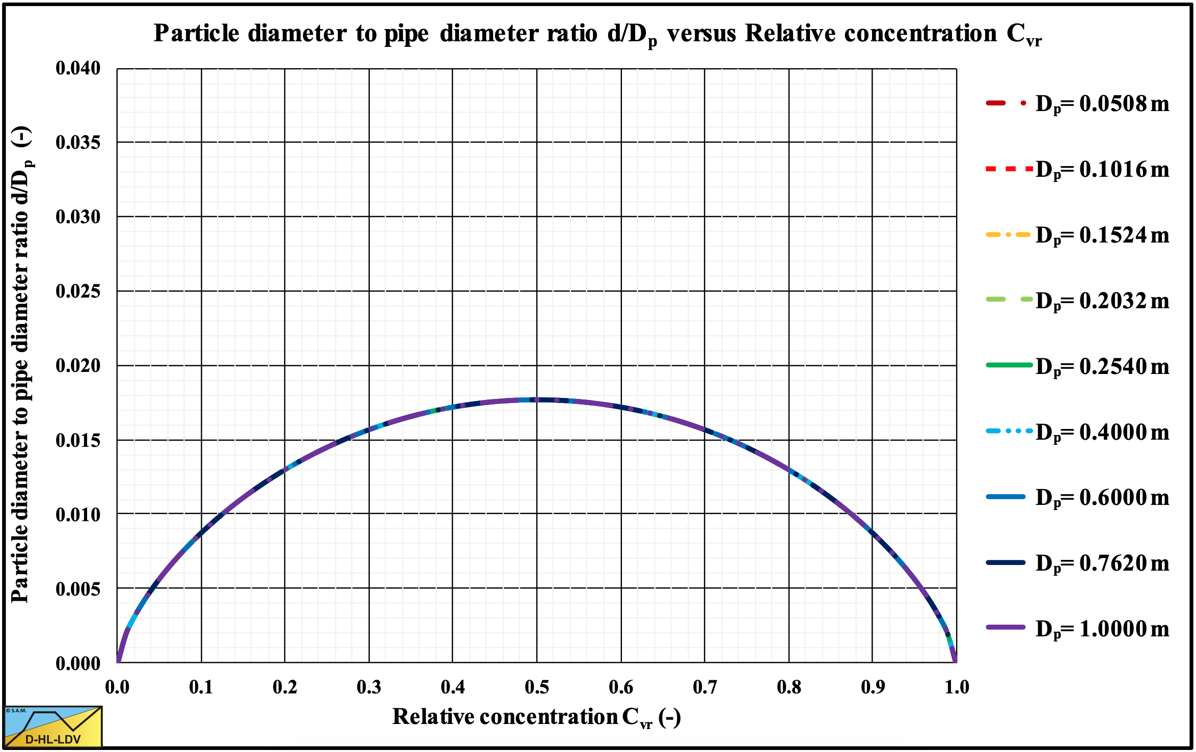
Figure 7.7-13 shows a particle diameter to pipe diameter ratio in the relative concentration range of 0.2-0.8 (operational range) of 0.013-0.018, matching Sellgren & Wilson (2007) mentioning 0.015-0.018 in several publications. A fundamental derivation of Sellgren & Wilson (2007) could not be found, but it is remarkable how close equation (7.7-23) approaches these values. Adding the wall shear stress, equation (7.7-21), gives slightly smaller values for spheres. For sands and gravels larger values are found.
Since the Sliding Flow Regime only occurs for large particles, the drag coefficient is about 1 for sand particles and 0.445 for spheres. The shape coefficient is about 0.77 for sand particles and 1 for spheres.
Figure 7.7-14 shows the shear stress ratio for a specific case, which is used for the derivation of the semi-empirical equation. Figure 7.7-15 shows the resulting particle diameter to pipe diameter ratio. Apparently this ratio is not just a fixed number (0.015), but it depends strongly on the relative concentration. There is also a linear proportionality with the sliding friction coefficient, the bed concentration and the particle dragcoefficient and a reversed proportionality with the particle shape factor. The proportionality with the pipe diameter is weak, while the proportionality with the particle diameter is very weak. The latter 2 proportionalities are because of the influence on the shear stress ratio. The proportionality of the line speed is also because of the presence in the shear stress ratio. Since sliding flow occurs above the Limit Deposit Velocity, the LDV/LSDV ratio is used in the shear stress equation, however instead of the LDV any line speed can be chosen to see the effect.
Since the starting assumption that the terminal settling velocity equals the friction velocity on top of the bed is only indicative for the occurrence of suspension, Figure 7.7-15 is also indicative. For normal relative concentrations the particle diameter to pipe diameter ratio is between 0.03 and 0.04, roughly twice the value as used by Sellgren & Wilson (2007).
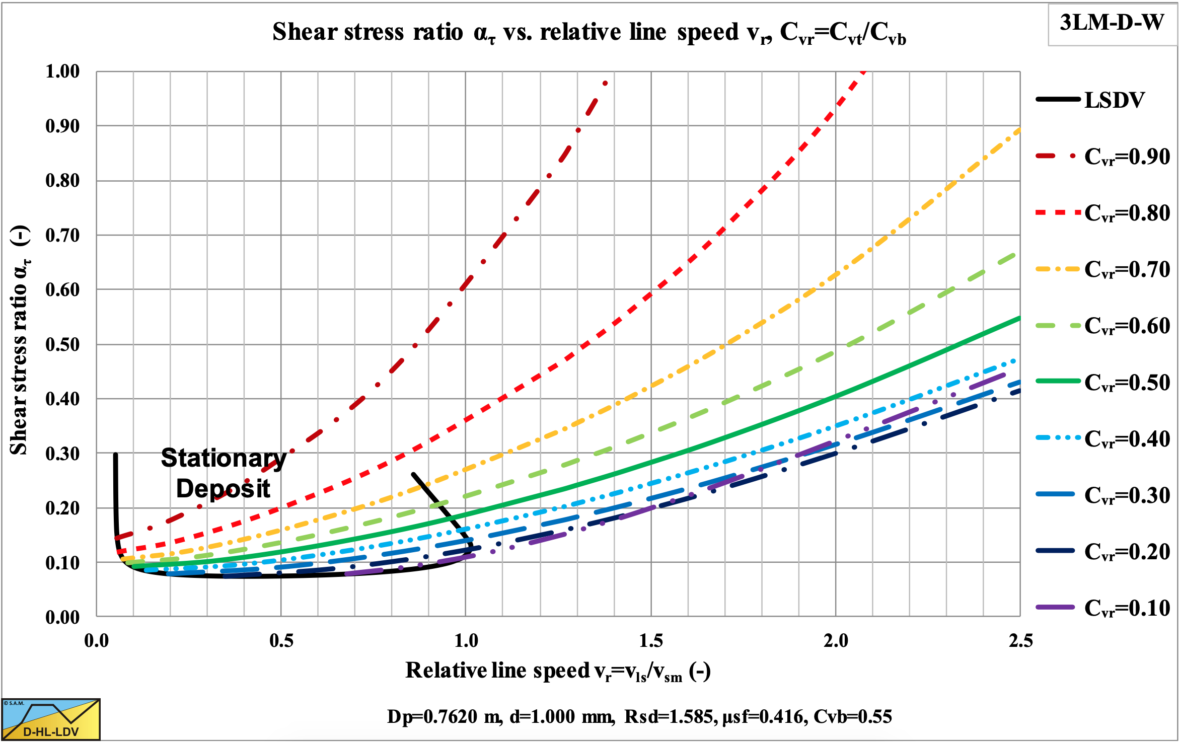
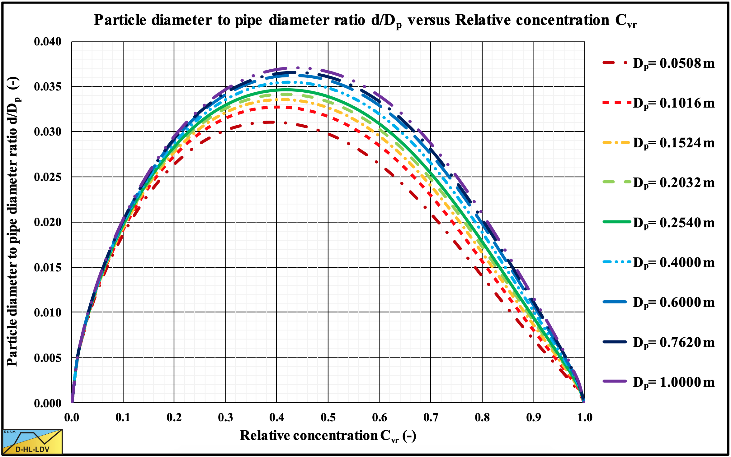
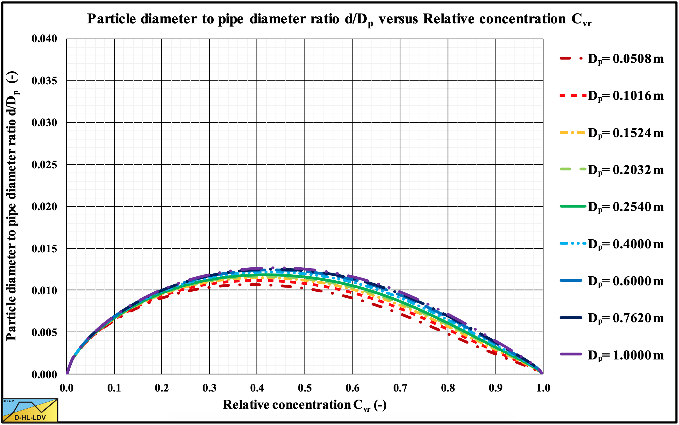
Figure 7.7-16 shows the particle diameter to pipe diameter ratio for spheres, which is much smaller than the ratio for natural sands and gravels. The peak value is close to the value of 0.015 as mentioned by Sellgren & Wilson (2007). The main reason for this is the smaller drag coefficient and the shape factor of 1. In equation (7.7-21).
For practical use and continuity half the theoretical diameter ratio is used as a start for sliding flow, while the transition from heterogeneous flow to sliding flow extends to twice the theoretical value found in Figure 7.7-15 and Figure 7.7-16.
For sands and gravels and relative volumetric concentrations close to 0.5, this gives a starting ratio of about rd/Dp=0.019 and full mobilization of sliding flow at rd/Dp=0.076. For spheres this gives a starting ratio of about rd/Dp=0.007 and full mobilization of sliding flow at rd/Dp=0.028. In both cases for a Dp=0.762 m pipe.
The order of magnitude of the diameter ratio matches the Sellgren & Wilson (2007) value of 0.015-0.018, however here it’s not a constant, but it is depending on many parameters.
7.7.6 Conclusions
The theoretical particle diameter to pipe diameter ratio matches the Sellgren & Wilson (2007) value of 0.015-0.018 for spheres if the pipe wall shear stress is not taken into account for medium relative volumetric concentrations. If the pipe wall shear stress is taken into account, slightly smaller values are found. For sand and gravel particles the values are roughly a factor 3 larger. This is mainly caused by the particle drag coefficient and the particle shape factor. Large spheres (which we consider here) have a drag coefficient of about 0.445 and a shape factor of 1. Sand and gravel particles have a drag coefficient of about 1 and a shape factor of about 0.77. For sands and gravels this of course depends on their shape.
Since spheres have a larger terminal settling velocity, the deposition is larger compared to sands and gravels. This results in a smaller particle diameter to pipe diameter ratio where the particles are not suspended anymore.
At very low (and high) relative concentrations the particle diameter to pipe diameter ratio is very small, implying that it is easy to have a thin layer of small particles at the pipe bottom. On the other hand, the sheet flow will dissolve this thin layer, resulting in a minimum relative concentration for the Sliding Flow Regime.
Since the assumption of terminal settling velocity equals the friction velocity is indicative, a transition from half the calculated ratio to double the calculated ratio is introduced, in order to have a smooth transition from the Heterogeneous Flow Regime to the Sliding Flow Regime.
7.7.7 Nomenclature Sliding Flow Regime
|
Ap |
Pipe cross section | m2 |
|
CD |
Particle drag coefficient |
- |
|
Cx |
Durand & Condolios particle Froude number |
- |
|
Cvt |
Delivered (transport) volumetric concentration | - |
|
Cvs |
Spatial volumetric concentration | - |
|
Cvb |
Bed concentration low line speeds | - |
|
CvB |
Bed/bottom concentration high line speeds, Sliding Flow Regime | - |
|
Cvr |
Relative spatial concentration Cvs/Cvb | - |
|
d |
Particle diameter | m |
|
Dp |
Pipe diameter | m |
|
Erhg |
Relative excess hydraulic gradient | - |
|
Erhg,HeHo |
Relative excess hydraulic gradient heterogeneous & homogeneous regimes |
- |
|
Erhg,SF |
Relative excess hydraulic gradient sliding flow regime |
- |
|
f |
Sliding Flow mobilization factor |
- |
|
FL |
Durand & Condolios LDV Froude number |
- |
|
g |
Gravitational constant 9.81 m/s2 |
m/s2 |
|
il |
Hydraulic gradient pure liquid |
m/m |
|
im |
Hydraulic gradient mixture |
m/m |
|
im,HeHo |
Hydraulic gradient heterogeneous & homogeneous regimes |
m/m |
|
im,SB |
Hydraulic gradient sliding bed regime |
m/m |
|
im,SF |
Hydraulic gradient sliding flow regime |
m/m |
|
L |
Length of pipe |
m |
|
LDV |
Limit Deposit Velocity |
m/s |
|
N |
Zandi & Govatos parameter |
- |
|
p |
Pressure |
kPa |
|
r |
Vertical coordinate in pipe starting at the bottom |
m |
|
rd/Dp |
Minimu particle diameter to pipe diameter ratio |
- |
|
Rsd |
Relative submerged density |
- |
|
u* |
Friction velocity |
m/s |
|
vls |
Line speed |
m/s |
|
vls,ldv |
Limit Deposit Velocity |
m/s |
|
vls,lsdv |
Limit of Stationary Velocity (start sliding bed) |
m/s |
|
vt |
Terminal settling velocity particles |
m/s |
| \(\ \alpha_{\tau} \) |
Shear stress ratio \(\ \tau_1/\tau_{12} \) |
- |
|
β |
Richardson & Zaki hindered settling power |
- |
|
β |
Bed angle with vertical |
rad |
|
ρl |
Carrier liquid density |
ton/m3 |
|
ρs |
Solids density |
ton/m3 |
| \(\ \tau_1 \) |
Pipe wall shear stress |
kPa |
| \(\ \tau_{12} \) |
Bed shear stress |
kPa |
|
μsf |
Sliding friction factor |
- |
|
ψ |
Shape factor (volume particle/volume sphere) |
- |