6.2: Early History

6.2.1 Blatch (1906)

The first experiments discovered were carried out by Nora Stanton Blatch (1906), with a pipeline of 1 inch and sand particles of d=0.15-0.25 mm and d=0.4-0.8 mm. She used two types of pipes, copper pipes and galvanized steel pipes.

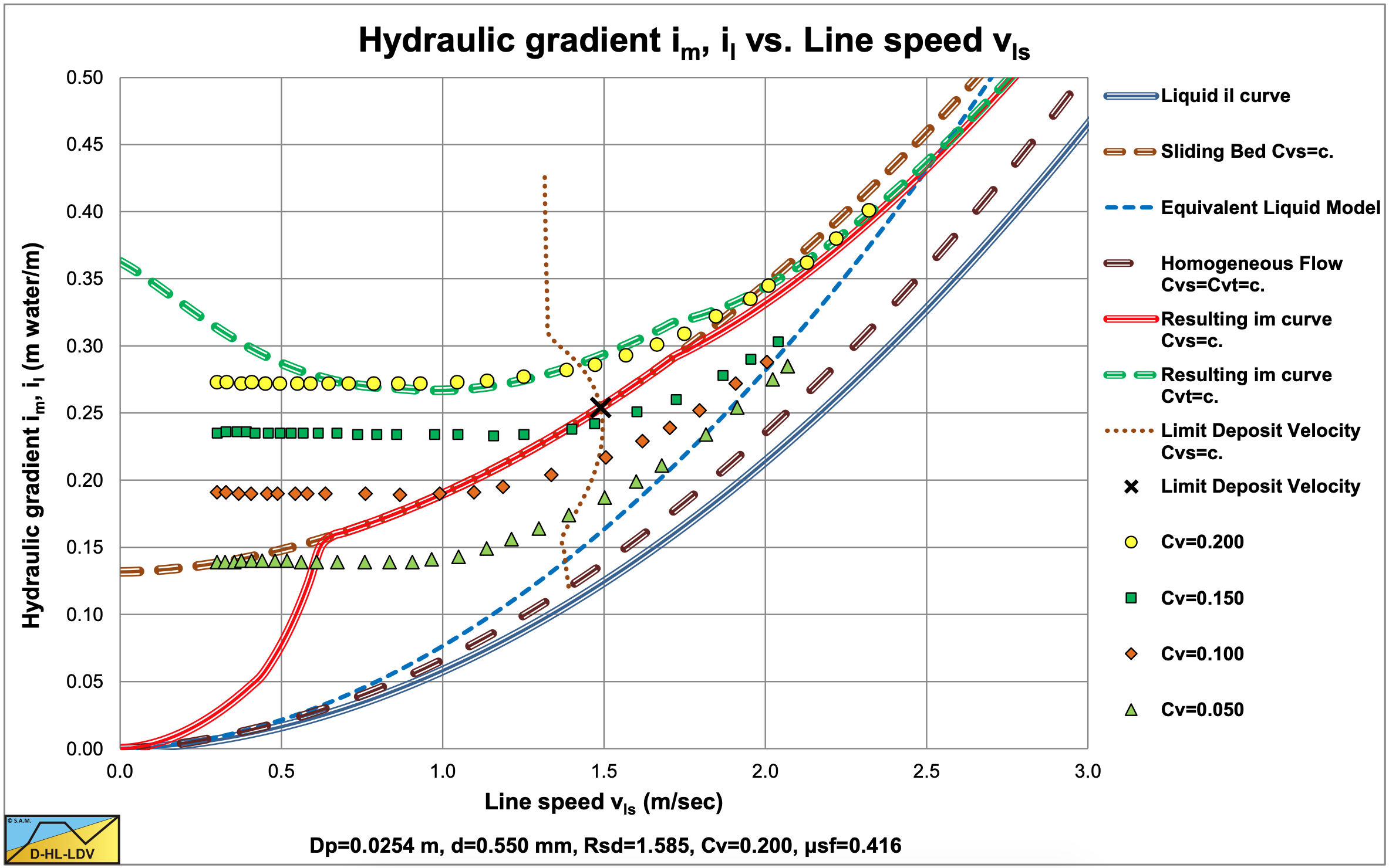
The experiments with the d=0.15-0.25 mm sand were carried out using the copper pipe. The results, digitized from a fit line graph (so not the original data points), are shown in Figure 6.2-1. At low line speeds the hydraulic gradient curve is horizontal (small C_vt) or decreasing (larger C_vt) with increasing line speed. It seems the curves have a minimum near a line speed of 1 m/sec and increase with a further increasing line speed, approaching the liquid curve. It is however not clear whether the curves asymptotically reach the liquid curve or the Equivalent Liquid Model (ELM) curves, or somewhere in between.

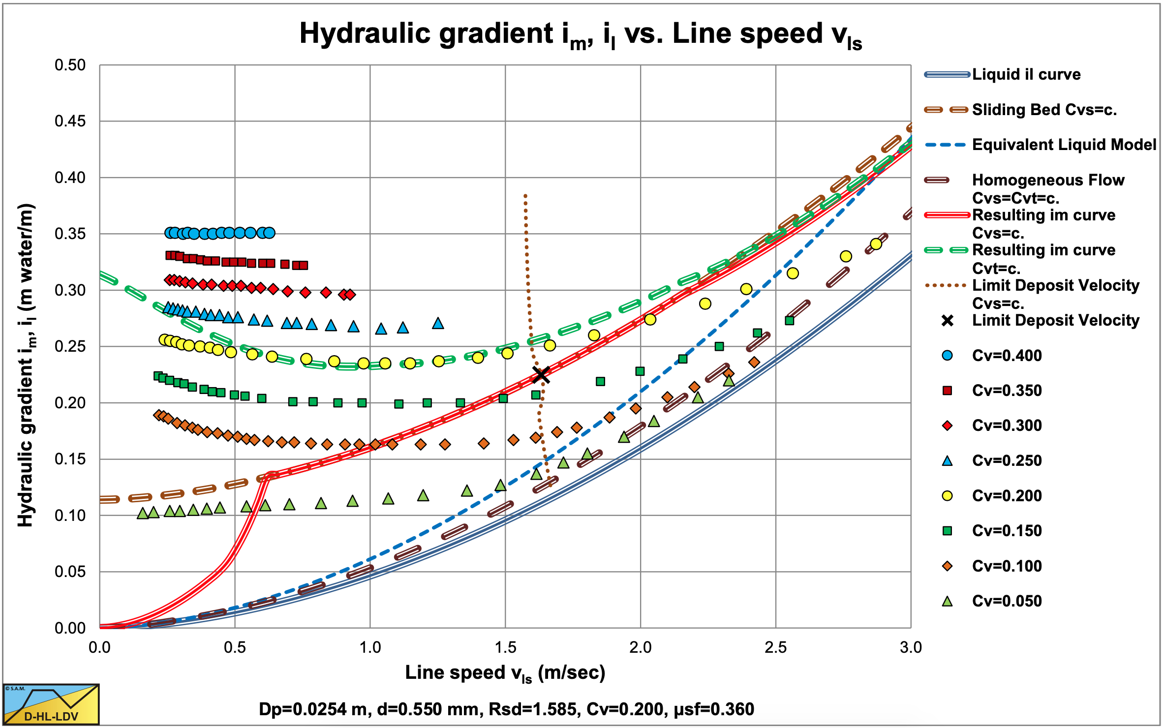
The first experiments with the d=0.4-0.8 mm sand were also carried out using the copper pipe. The results, digitized from a fit line graph (so not the original data points), are shown in Figure 6.2-2. At low line speeds the hydraulic gradient curve is almost horizontal with increasing line speed. This makes the minimum hard to find. At higher line speeds the curves approach the clean water curves asymptotically.

The second set of experiments with the d=0.4-0.8 mm sand were carried out using the galvanized steel pipe. The results, digitized from a fit line graph (so not the original data points), are shown in Figure 6.2-3. At low line speeds the hydraulic gradient curve is almost horizontal with increasing line speed. This makes the minimum hard to find. At higher line speeds the curves approach the clean water curves asymptotically, but less than in the copper pipe. The clean water curve is clearly much steeper than with the copper pipe, due to the wall roughness.

It looks like very small particles (d=0.2 mm) tend to have ELM behavior at high line speeds, while medium sized particles (d=0.55 mm) approach the clean water curve. The experiments did not contain large particles, so their behavior is not investigated. This behavior depends on many parameters, so one can only draw conclusions for the values of the parameters tested.

Figure 6.2-1: Sand with d=0.15-0.25 mm in a 1 inch diameter copper pipe.
Data points of Blatch (1906) reconstructed from fit lines (source (Westendorp, 1948)).

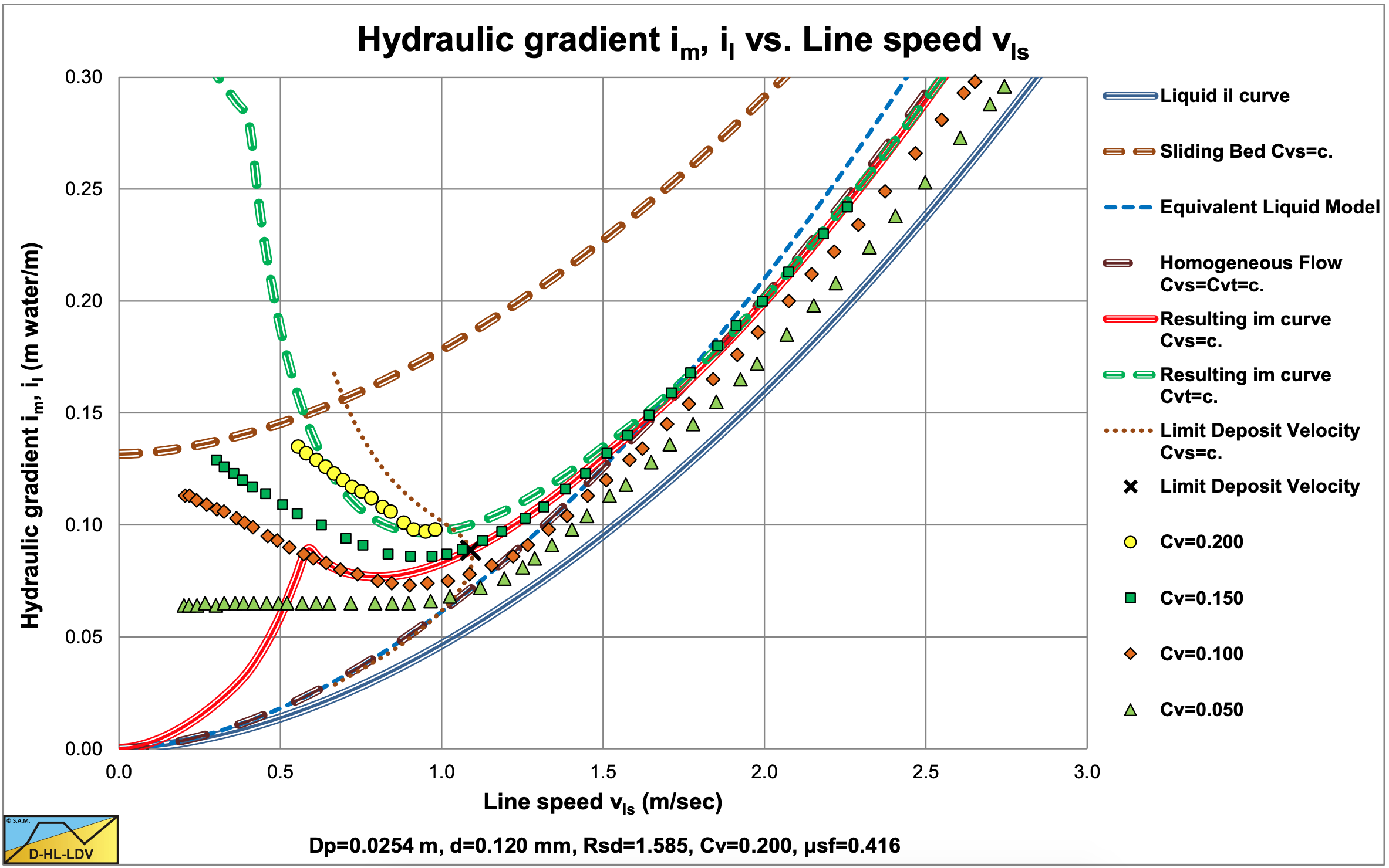
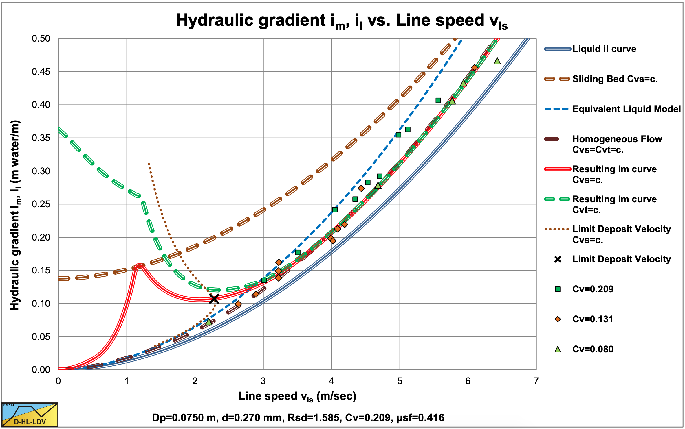
In Figure 6.2-1 the data are compared with the DHLLDV Framework for a particle diameter of d=0.12 mm and a volumetric concentration of 20%.

Figure 6.2-2: Sand with d=0.4-0.8 mm in a 1 inch diameter copper pipe.
Data points of Blatch (1906) reconstructed from fit lines (source (Westendorp, 1948)).

Figure 6.2-3: Sand with d=0.4-0.8 mm in a 1 inch diameter steel pipe.
Data points of Blatch (1906) reconstructed from fit lines (source (Westendorp, 1948)).

6.2.2 Howard (1938)

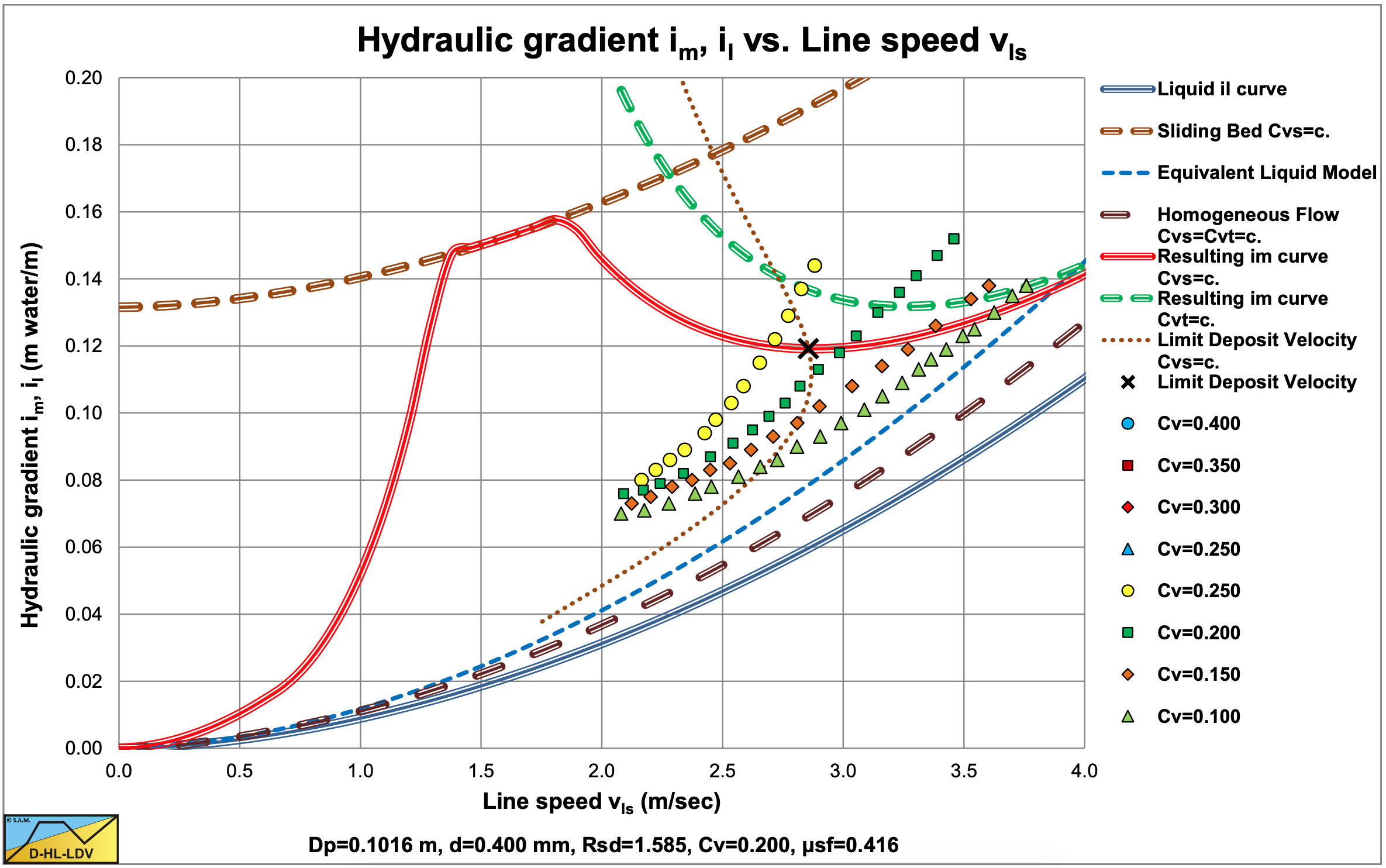
Howard (1938) carried out experiments with a d=0.4 mm graded sand (d=0.1-2.0 mm, 80%<0.8 mm) in a 4 inch pipe. The results, digitized from a fit line graph (so not the original data points), are shown in Figure 6.2-4. The hydraulic gradient curves start above a line speed of 2 m/sec and the distance (excess hydraulic gradient) with the liquid hydraulic gradient curve tends to be increasing with increasing line speed. This looks like following the ELM curves for the different concentrations. The curves are however steeper than the ELM curves, which is not observed with any other experiments. An explanation could be that the concentration definition used by Howard (1938) is not the volumetric delivered concentration, but he may have used another definition. The data from the trend lines do not show any resemblance with the DHLLDV Framework.

6.2.3 Siegfried (Durepaire, 1939)

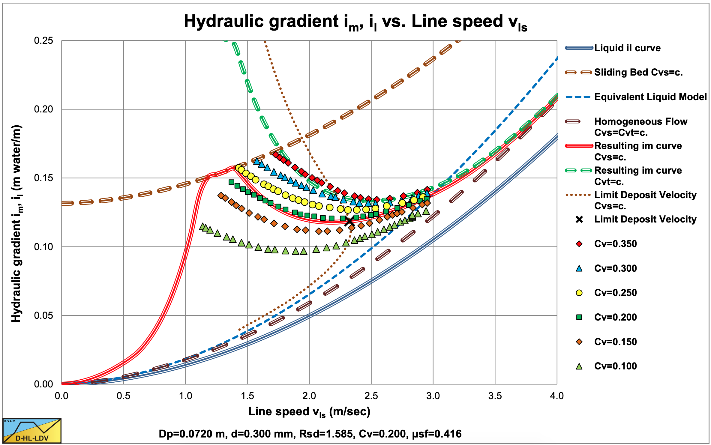
Siegfried (Durepaire, 1939) carried out experiments with a d=0.3 mm sand in a 0.072 m diameter pipe. The results, digitized from a fit line graph (so not the original data points), are shown in Figure 6.2-5. The hydraulic gradient curves decrease with an increasing line speed at low line speeds, up to a minimum of the hydraulic gradient curves, after which they increase approaching the liquid hydraulic gradient curve asymptotically.

The magnitude of the hydraulic gradients in the original graph however is too small compared to the experiments of others. An explanation could be that the concentration definition used by Siegfried (Durepaire, 1939) is not the volumetric spatial concentration, but he may have used another definition. Another explanation is that the values on the axis of the graphs, a copy of a copy, were not correct. Figure 6.2-5 is a modified version of the original graph, but the shapes of the hydraulic gradient curves have not changed.

6.2.4 O’Brien & Folsom (1939)

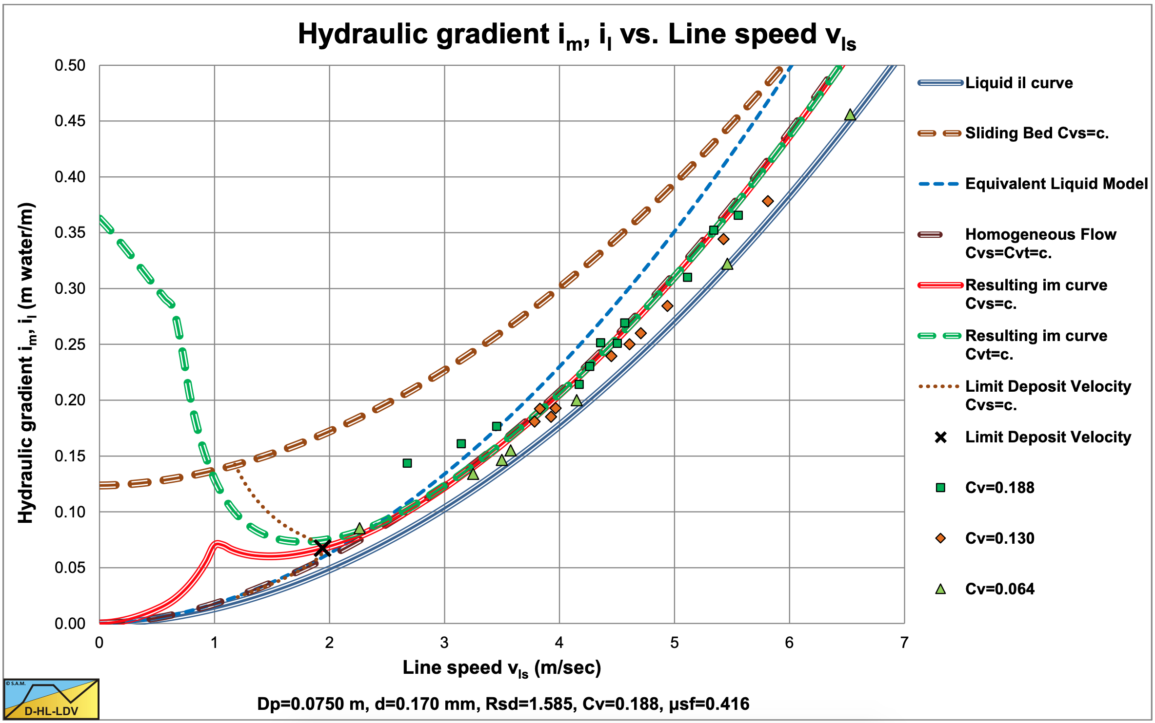
O’Brien & Folsom (1939) carried out experiments with two sands, d=0.17 mm and d=0.27 mm in a 2 inch and a 3 inch pipe. In their original graphs, the hydraulic gradient is expressed in meters mixture per meter pipe length. The original graph also contains the volumetric concentration of each data point. By recalculating the real hydraulic gradients and grouping the data points in concentration ranges, Figure 6.2-6 and Figure 6.2-7 are constructed. The concentrations in the legends are the average values of the concentration ranges, so some scatter may be expected. Figure 6.2-6 shows a more or less homogeneous behavior. Most data points are in between the ELM curve and the clean water curve. It should be mentioned that the figure only gives the ELM curve for C_v=0.188. The data points are closer to the ELM curve than to the clean water (liquid) curve. Figure 6.2-7 shows the same behavior, but the data points are closer to the ELM curve.

Figure 6.2-4: Sand with d=0.4 mm in a 4 inch diameter pipe.
Data points of Howard (1938) reconstructed from fit lines (source (Westendorp, 1948)).

Figure 6.2-5: Sand with d=0.30 mm in a 0.072 m diameter pipe.
Data points of Siegfried (Durepaire, 1939) reconstructed from fit lines (source (Westendorp, 1948)).

Figure 6.2-6: The data of O’Brien & Folsom (1939) for d=0.17 mm processed.

Figure 6.2-7: The data of O’Brien & Folsom (1939) for d=0.27 mm processed.

6.2.5 Conclusions & Discussion Early History

This chapter is based on an old Dutch report of Westendorp (1948) with additions and modifications of the author and gives the state of the art of slurry transport research up to 1948.

The available experimental data can be divided into two groups, laboratory tests with pipes with a diameter of 2 to 6 inch and full scale tests with pipes with diameters of 0.50 to 0.85 m. The laboratory tests resulted in reasonable data, the full scale tests did not. Reasonable in this case means reproducible data. The data published are limited, meaning that each researcher used one or two pipe diameters and one or two particle diameters. The variation of the line speed was also limited. It is thus not possible to draw quantitative conclusions, but some qualitative conclusions will be discussed.

The flow of water through pipes is influenced by the physical properties of the liquid (viscosity and density) and the geometry of the pipe (diameter and roughness). The flow of sand or gravel with water as the carrier liquid, the physical properties of the solids (density, size, shape, etc.) also play a role. The solids do not have to form a homogeneous mixture with the liquid and may have a behavior that does not follow the hydraulical laws.

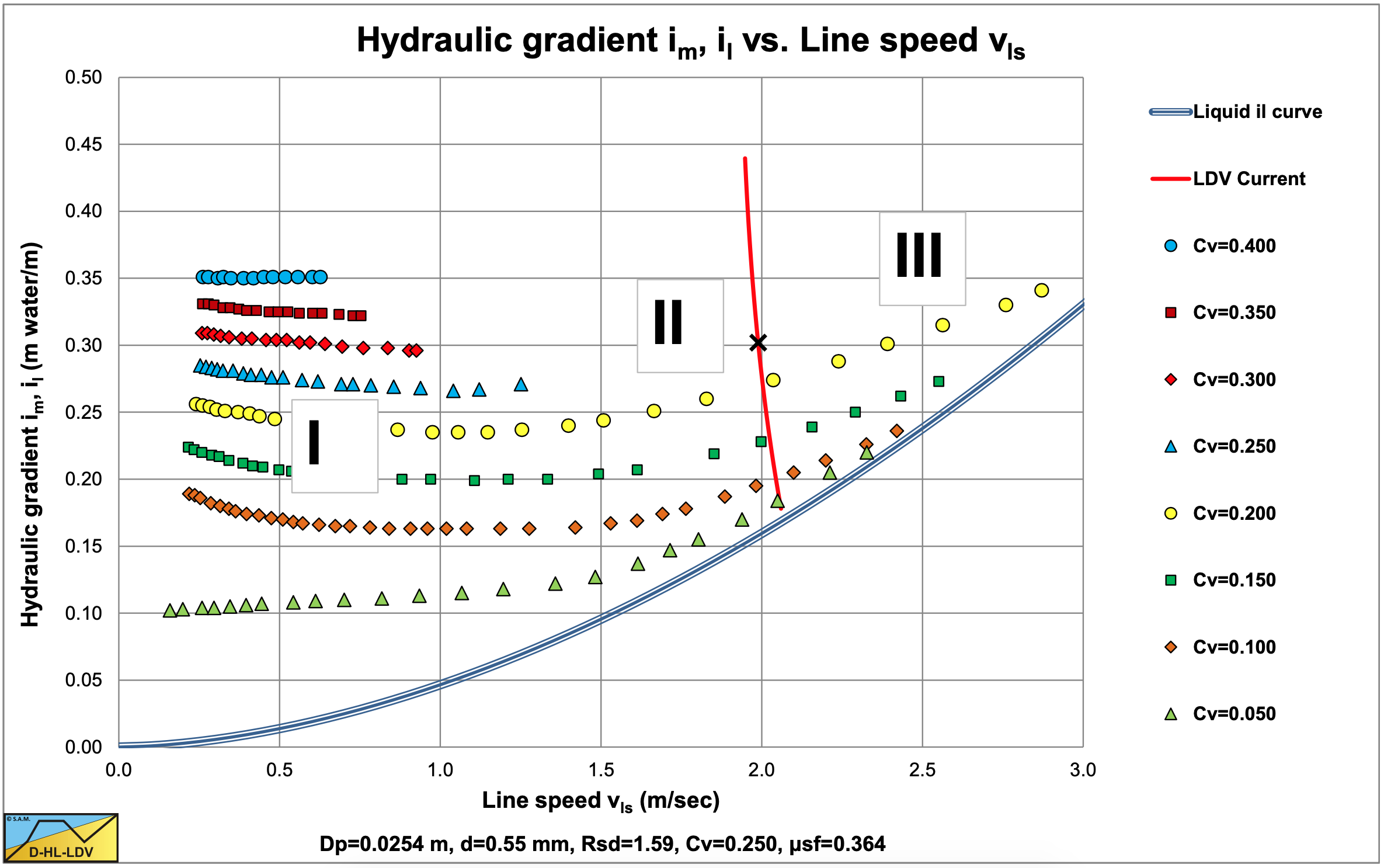
Figure 6.2-1, Figure 6.2-2, Figure 6.2-3, Figure 6.2-4, Figure 6.2-5, Figure 6.2-6 and Figure 6.2-7 show a characteristic behavior of the hydraulic gradient versus the line speed. Going from left to right (increasing line speed) the curves are first almost horizontal or decreasing (region I), followed by a transition region (region II), after which the hydraulic gradient will increase and approach the liquid hydraulic gradient (region III). The transition of region II to region III is often named the Limit Deposit Velocity (LDV). In region III almost all solids particles will be in suspension and form a more or less homogeneous liquid. Below the LDV particles will form a bed, fixed or sliding. At higher velocities this particle transport will be a saltating transport. At the lower velocities there will be a bed with particles moving and rolling on top of the bed (sheet flow). The definition of the LDV is very important, since in literature also the transition fixed bed to sliding bed is often used in 2LM and 3LM models. This transition is named here the limit of stationary deposit velocity (LSDV).

Figure 6.2-8: The regions I, II and III.

So below the LDV there are two types of transport in the pipe:

1. The liquid with the solids in suspension, behaving as a homogeneous liquid.
2. The solids at the bottom of the pipe, not following fluid mechanical laws.

These two types of transport are interrelated. If there is a deposit at the bottom, the real velocity above a bed (deposit) will differ from the cross section averaged line speed. The real velocity above the bed is larger than the line speed.

Region I: The general direction of the hydraulic gradient versus line speed curve is either horizontal or decreasing with increasing line speed, if constant delivered concentration curves are considered. An appropriate physical explanation for this behavior was not yet given in 1948. Some authors suggest that with a decreasing line speed, the bed will occupy part of the pipe cross section in such a way that the velocity above the bed is constant, so equal to the LDV. When the bed height is increasing with decreasing line speed, the bed surface will increase and this the resulting roughness for the flow above the bed, also resulting in a decreasing hydraulic radius, influencing the Darcy-Weisbach friction factor. A further decrease of the line speed may lead to pipe blockage or clogging.

Region II: Is a transition region between region I (fixed or sliding bed) and region III (homogeneous transport). This region is often referred to as heterogeneous transport. For sand suspensions this region is small, however Blatch (1906) stated that this region is small for uniform sands and gets bigger for graded sand, the more graded the bigger. Siegfried (Durepaire, 1939) observed that the curve, given a certain delivered concentration, is higher with increasing line speed than with decreasing line speed. Apparently, removing a fixed or sliding bed (bringing it into suspension) takes more energy than the opposite action, a sort of hysteresis. Region II also contains the point of minimum hydraulic gradient. According to Howard (1938) this happens when the deposit (bed) is completely removed, which is defined as the LDV. The LDV increases with increasing concentration and increasing particle size.

Region III: This region contains the physical situation where the solid-liquid mixture is assumed to be (pseudo) homogeneous. Homogeneous is defined as a transport with a symmetrical velocity distribution with respect to the center of the horizontal pipe and a uniform concentration distribution. Because of gravity, the concentration in the lower half of the pipe will always be higher than in the upper half of the pipe, so real homogeneous transport according to the definition will never occur. With fine sand, the hydraulic gradient curves at high line speeds will approach the clean water curve with increasing line speed. With coarser sand the mixture hydraulic gradient will be larger than the liquid hydraulic gradient. According to O’Brien & Folsom (1939) the larger the particles, the larger the mixture hydraulic gradient. This increase in mixture hydraulic gradient of course depends on the solids concentration.

Vaughn (Howard, 1939) posed that the hydraulic gradient also depends on the viscosity of the mixture and of some characteristic particle size. Dent (Howard, 1939) states that at very high line speeds the hydraulic gradient will deviate from the clean water curve, increase with respect to the liquid hydraulic gradient, but he did not explain this. Wilson (1942) and Danel (Howard, 1939) give an explanation for the observation that with fine sand the mixture hydraulic gradient is lower than the liquid hydraulic gradient. They assume that fine particles influence the occurrence of the small eddies due to turbulence, resulting in less energy dissipation. The particles have to be smaller than the size of the eddies. This will occur for particles with a settling velocity in the Stokes region (d<0.1 mm). Larger particles will not result in such behavior. O’Brien & Folsom (1939) found that at high line speeds and small particles the behavior almost follows the Equivalent Liquid Model.

The Limit Deposit Velocity (LDV): The LDV is not defined clearly. Usually the LDV is defined as the line speed above which all the particles are in suspension or as the line speed above which the mixture hydraulic gradient equals the liquid hydraulic gradient. The LDV increases strongly with an increasing delivered volumetric concentration. The LDV also increases with an increasing particle size, with an increasing pipe diameter and with a decreasing pipe wall roughness. Durepaire (1939) assumes a proportionality between the LDV and the delivered concentration to a power less than 0.5. Franzi (1941) gives a second degree function. The relative submerged density of the solids does not have much influence on the LDV in small diameter pipes (D_p<0.2 m), but it does in larger diameter pipes. The LDV will increase with an increasing relative submerged density.

Characteristics of the solids: In 1948 it was not yet clear, which solids characteristics should be used for the determination of the solids effect in slurry flow through pipes. Often the particle size distribution graphs (PSD) are mentioned, but also the relative submerged density, the porosity and the type of material. O’Brien & Folsom (1939) and Wilson (1942) added the terminal settling velocity to this list.

Particle size: Often the PSD is complemented with a mean particle diameter or some other characteristic diameter (for example the d₁₀). Dent (Howard, 1939) does not support the effective particle size as proposed by Howard (1938). The effect of 15% gravel is much larger than the effect of 25% sand. Coarse material has much more influence than fine material. A better characteristic diameter would be the d₂₅. Vaughn (Howard, 1939) states that the ratio of the particle diameter to the pipe diameter is of importance. Franzi (1941) mentions that adding some very fine particles to coarse particles will sometimes reduce the hydraulic gradient. It is thus difficult to find a good characteristic particle diameter.

Terminal settling velocity: From many observations it is clear (Howard, 1938) that the distribution of the particles in a cross section of the pipe is not uniform. On average, the concentration increases towards the bottom of the pipe. O’Brien & Folsom (1939) draw the conclusion that the terminal settling velocity of the particles is the most dominant characteristic the solids. The PSD, relative submerged density, porosity and other parameters are only important in order to quantify the terminal settling velocity. They measure this terminal settling velocity by testing the settling velocity of each fraction in clean water and determining the highest settling velocity of the fraction. Whether or not they take hindered settling into account is not clear. Vaughn (Howard, 1939) remarks that it may be important to determine the settling velocity of a sand-mud mixture, which looks more like reality, probably giving smaller values for the settling velocity.

Modeling: Wilson (1942) assumes that particles in suspension will, on average, keep their vertical position in the flow, also assuming a constant spatial concentration distribution in the pipe cross section. Now suppose particles settle with a terminal settling velocity vt and are pushed up again by lift forces. This means that the fluid will carry out work to compensate for the loss of potential energy. This work will be larger than the potential energy alone, because there is also a loss of mechanical energy due to viscous friction, both for descending and ascending particles. Wilson (1942) derived the following equation:

\[\ \mathrm{i}_{\mathrm{m}}=\mathrm{i}_{\mathrm{l}}+\mathrm{K} \cdot \frac{\mathrm{C}_{\mathrm{m} \mathrm{s}} \cdot \mathrm{v}_{\mathrm{t}}}{\mathrm{v}_{\mathrm{l} \mathrm{s}}}=\frac{\lambda_{\mathrm{l}} \cdot \mathrm{v}_{\mathrm{l} \mathrm{s}}^{2}}{2 \cdot \mathrm{g} \cdot \mathrm{D}_{\mathrm{p}}}+\mathrm{K} \cdot \frac{\mathrm{C}_{\mathrm{m} \mathrm{s}} \cdot \mathrm{v}_{\mathrm{t}}}{\mathrm{v}_{\mathrm{ls}}}=\frac{\lambda_{\mathrm{l}} \cdot \mathrm{v}_{\mathrm{ls}}^{2}}{2 \cdot \mathrm{g} \cdot \mathrm{D}_{\mathrm{p}}} \cdot\left(\mathrm{1}+\mathrm{2} \cdot \mathrm{K} \cdot \frac{\mathrm{C}_{\mathrm{m} \mathrm{s}} \cdot \mathrm{v}_{\mathrm{t}} \cdot \mathrm{g} \cdot \mathrm{D}_{\mathrm{p}}}{\lambda_{\mathrm{l}} \cdot \mathrm{v}_{\mathrm{l} \mathrm{s}}^{\mathrm{3}}}\right)\]

The coefficient K is a proportionality coefficient, C_ms is the concentration by weight, v_t the terminal settling velocity and v_ls the line speed. With an increasing line speed, the mixture hydraulic gradient will approach the liquid hydraulic gradient asymptotically. For a certain mixture and pipe diameter, there will be a line speed where the mixture hydraulic gradient has a minimum. This minimum is at the line speed:

\[\ \mathrm{v}_{\mathrm{l s}, \mathrm{m i n}}^{\mathrm{3}}=\mathrm{K} \cdot \frac{\mathrm{C}_{\mathrm{m s}} \cdot \mathrm{v}_{\mathrm{t}} \cdot \mathrm{g} \cdot \mathrm{D}_{\mathrm{p}}}{\lambda_{\mathrm{l}}}\]

Substituting this solution for the minimum hydraulic gradient line speed gives:

\[\ \mathrm{i}_{\mathrm{m}}=\mathrm{3} \cdot \mathrm{i}_{\mathrm{l}}=\mathrm{3} \cdot \frac{\lambda_{\mathrm{l}} \cdot \mathrm{v}_{\mathrm{l s}, \mathrm{m i n}}^{\mathrm{2}}}{\mathrm{2} \cdot \mathrm{g} \cdot \mathrm{D}_{\mathrm{p}}}\]

In other words, at the minimum hydraulic gradient line speed, the mixture hydraulic gradient is always equal to 3 times the liquid hydraulic gradient, assuming constant values for the other parameters in the equation. Applying this theory on the experiments of Blatch (1906), requires K values between 2 and 10. The maximum K value was found at the minimum hydraulic gradient line speed. A further increasing line speed reduces the K value to a value of 1. It would be interesting to find a fundamental equation for this K value. Lorentz in the discussion on Wilson (1942) disagrees with the above equation. He feels its adding up energy losses, without looking at possible interactions. The two terms in equation (6.2-1) deal with different phases of the problem. The first term deals with the Darcy-Weisbach friction of clean water, the second term with the turbulent energy required to keep the particles in suspension. The energy in the second term could occur in the first term as Darcy-Weisbach friction and in the second term as potential energy. From some measurements of Wilson (1942) this seems to be the case. So equation (6.2-1) does not give a full explanation of the problem, but it’s a first reasonable description. Dent (1939) gives a similar equation, which is discussed later.

Blatch (1906) gives for the minimum mixture hydraulic gradient line speed (the economical line speed) some rules of the thumb. For a 1 inch pipe per 1000 m of pipe length the pressure loss is the pressure loss of the liquid at 1 m/s line speed plus 9.6 m.w.c for every 1% of delivered volumetric concentration. For a 32 inch pipe per 1000 m of pipe length the pressure loss is the pressure loss of the liquid at 3 m/sec line speed plus 1.2 m.w.c. for every 1% of delivered volumetric concentration. She also gave the following information:

Table 6.2-1: Some characteristic velocities according to Blatch (1906).

Pipe diameter	Line speed giving blockage	Economical line speed	LDV all particles in suspension
1 inch	0.38 m/sec	1.07 m/sec	2.4-2/7 m/sec
2 inch	0.76 m/sec	1.22 m/sec	-
32 inch	1.8-2.1 m/sec	2.75 m/sec	4.3 m/sec

Table 6.2-2: The LDV values measured by Blatch (1906), source Graf et al.(1970).

Blatch (1906)	Dp=0.0254 m
d in mm	d in m	Archimedes	LDV in m/sec	FL
0.20	0.00020	102	0.94	1.04
0.20	0.00020	102	0.92	1.01
0.20	0.00020	102	0.96	1.06
0.55	0.00055	2125	1.26	1.39
0.55	0.00055	2125	1.06	1.17
0.55	0.00055	2125	1.01	1.12
0.55	0.00055	2125	0.96	1.06
0.55	0.00055	2125	1.31	1.44
0.55	0.00055	2125	1.29	1.42

It looks like the LDV values in Table 6.2-2 are in fact the economical line speeds measured by Blatch (1906).

Plugging the line: Decreasing the line speed at a certain delivered concentration will result in an increasing deposit (bed height) until the pipe is blocked completely. If at a low line speed, the delivered concentration is increased, then a certain delivered concentration will also result in pipe blockage. This pipe blockage will occur at higher line speeds if the particles are coarser. Fine particles will result in a smoother bed making rolling transport easier. According to Durepair (1939) this blockage is also determined by the stability of the flow, thus from the interaction between the pump and the mixture flow through the pipeline. According to O’Brien & Folsom (1939) the amount of solids in suspension depend on the amount of turbulence in the pipe. An increase of this turbulence will increase the allowable concentration delivered. A pump will cause more turbulence close behind the pump resulting in a lower probability of blockage than further in the pipeline. If the concentration is suddenly increased, then close behind the pump there will not be blockage, but further in the pipeline this may cause blockage.

The above summary of the state of the art is not the opinion of the author, but it is what was found in literature up to 1948. This is the starting point for the later researchers and puts their findings in a historical perspective.
The concept of Wilson (1942) of using a potential energy approach in order to explain the solids effect of the energy losses is a concept which is also used by Newitt et al. (1955) and more recently by Miedema & Ramsdell (2013), combined with kinetic energy losses. Many researchers developed a hydraulic gradient or pressure loss equation consisting of a Darcy-Weisbach friction term and a second term for the solids effect, usually the latter reversely proportional to the line speed. The equation of Wilson (1942) in this respect is also very similar to the equation of Fuhrboter (1961), assuming that the terminal settling velocity equals about 100 time times the particle diameter for fine and medium sands.

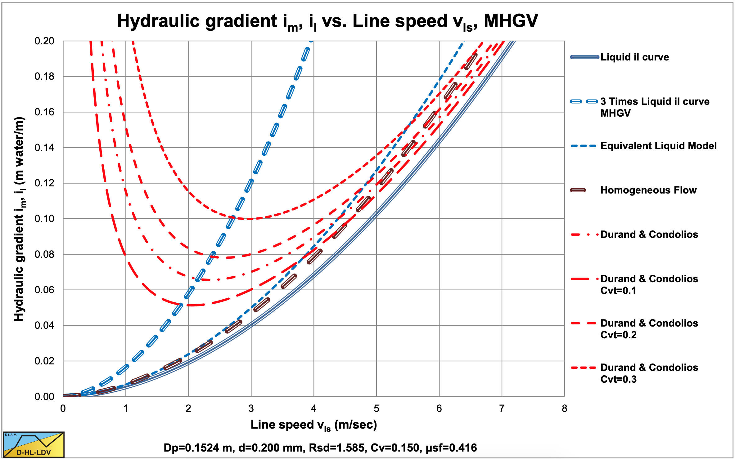
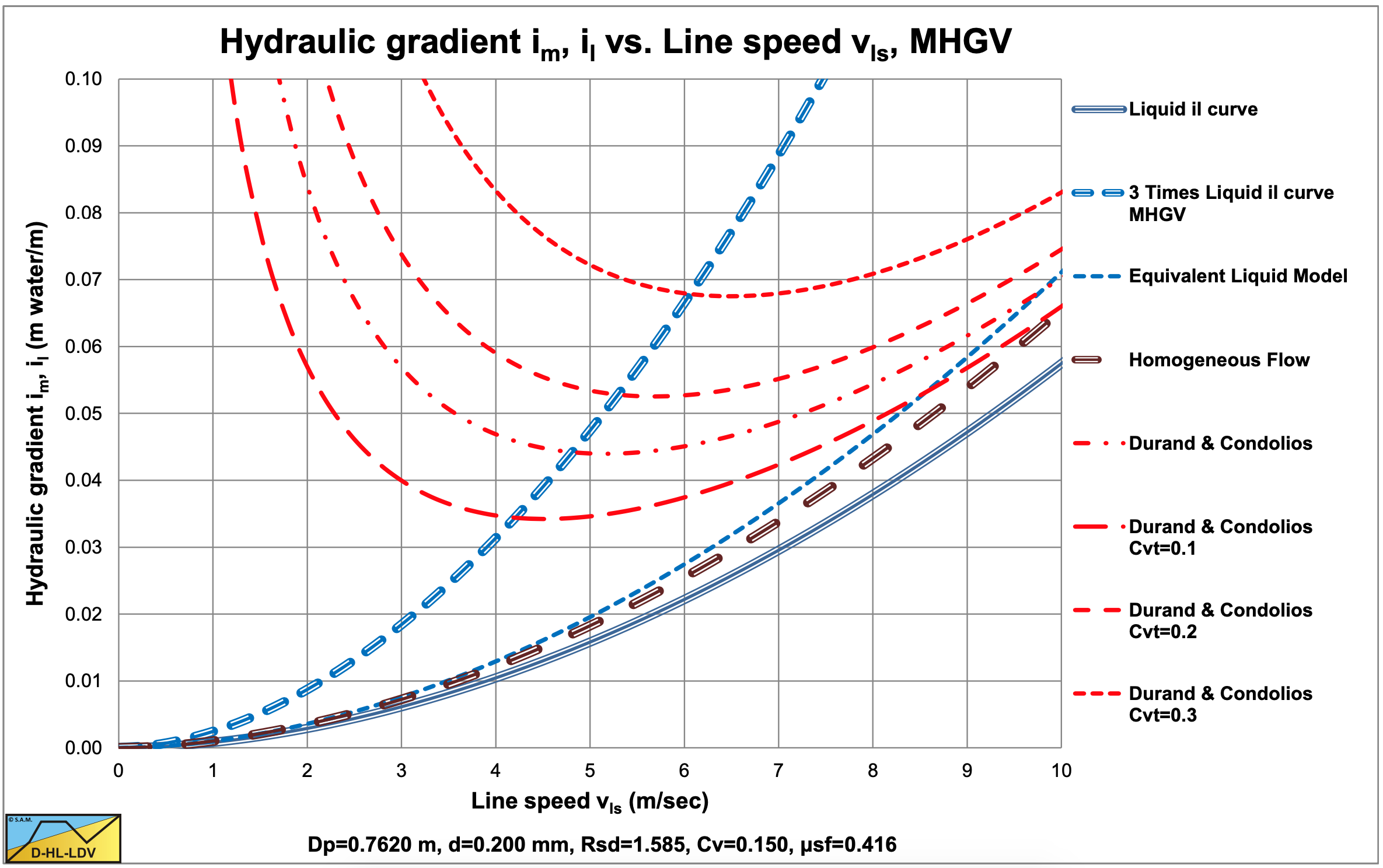
At high line speeds a certain range of particle diameters will result in a curve approaching the liquid curve, while other particle diameters result in a curve approaching the ELM curve.
The concept of the minimum hydraulic gradient velocity (MHGV) gives the basis for a graphical representation of this line speed. In a hydraulic gradient versus line speed graph, 3 curves have to be drawn, the liquid hydraulic gradient curve, 3 times this curve and the mixture hydraulic gradient curve. The intersection point of the mixture hydraulic gradient curve and the 3 times the liquid hydraulic gradient curve is the minimum hydraulic gradient point.

Figure 6.2-9 and Figure 6.2-10 show the MHGV curve for 4 concentrations and 2 pipe diameters. The mixture hydraulic gradient curves are based on the Durand & Condolios (1952) model. The fact that the MHGV curves seem to be a little on the left of the minimum points of the mixture hydraulic gradient curves is the result of a line speed dependent Darcy Weisbach friction factor. In the derivation resulting in 3 times the liquid hydraulic gradient curve, this friction factor is considered a constant.

Figure 6.2-9: The MHGV curve for a d=0.2 mm particle in a D_p=0.1524 m (6 inch) pipe.

Figure 6.2-10: The MHGV curve for a d=0.2 mm particle in a D_p=0.762 m (30 inch) pipe.