6.5: The Newitt et al. (1955) Model

Newitt et al. (1955) carried out experiments in a 1 inch pipe with sands of 0.0965 mm, 0.203 mm, 0.762 mm and gravel of 4.5 mm. They also carried out experiments with gravel of 3.2-6.4 mm, coal of 3.2-4.8 mm (R_sd =0.4) and MnO2 of 1.6-3.2 mm (R_sd =3.1). Newitt et al. (1955) distinguished a heterogeneous regime and a sliding bed regime.

6.5.1 The Heterogeneous Regime

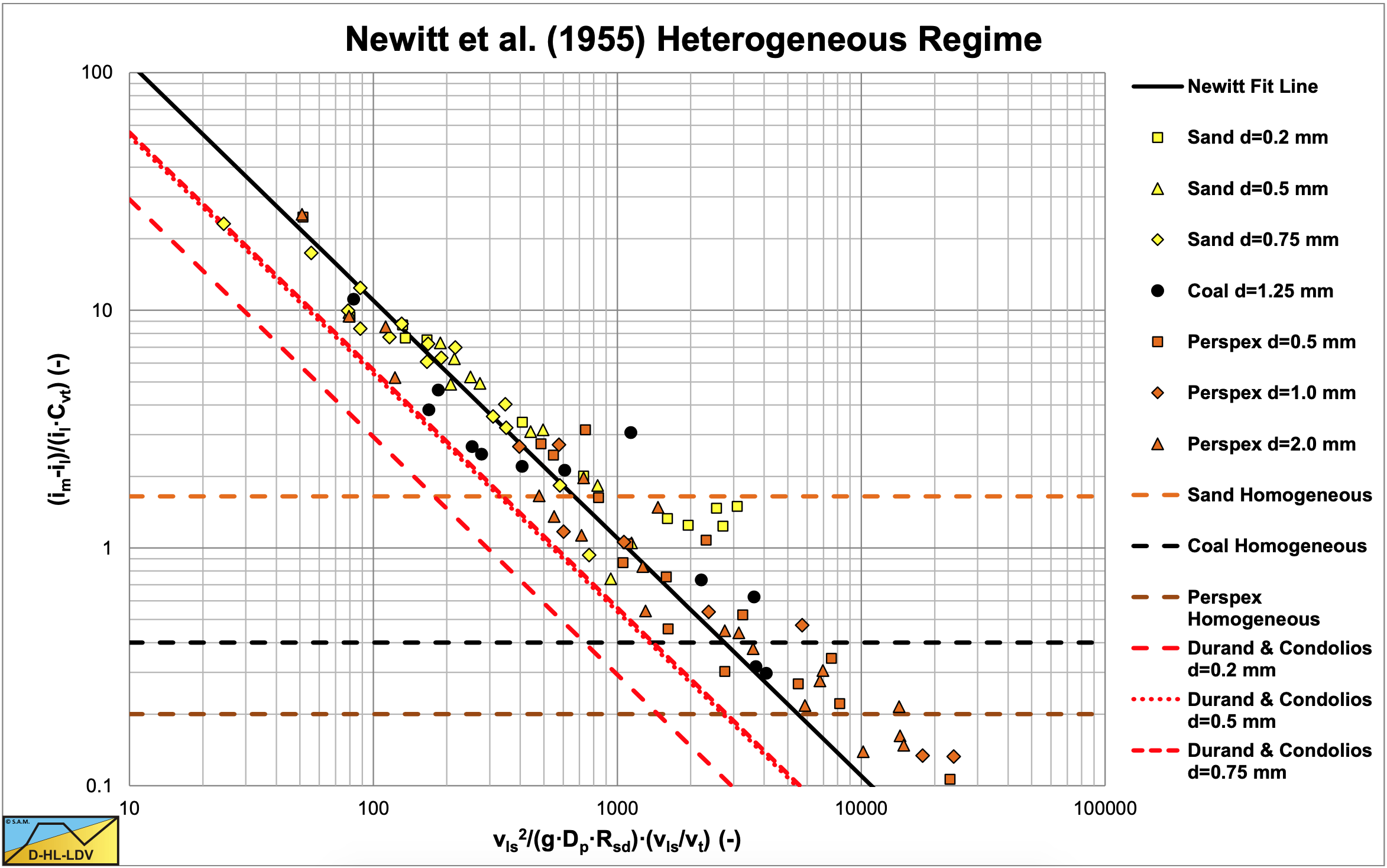
For the heterogeneous regime they assumed that the energy loss due to the solids is based on keeping the particles floating. In other words, due to gravity the particles will move down continuously and the energy required moving them up, the potential energy, results in an excess pressure loss. Based on the conservation of potential energy of the particles the following equation is derived:

\[\ \begin{array}{left}\Delta \mathrm{p}_{\mathrm{m}}=\Delta \mathrm{p}_{\mathrm{l}} \cdot\left(\mathrm{1}+\mathrm{K}_{\mathrm{1}} \cdot\left(\mathrm{g} \cdot \mathrm{D}_{\mathrm{p}} \cdot \mathrm{R}_{\mathrm{s d}}\right) \cdot \mathrm{v}_{\mathrm{t}} \cdot \mathrm{C}_{\mathrm{v t}} \cdot\left(\frac{\mathrm{1}}{\mathrm{v}_{\mathrm{l s}}}\right)^{3}\right)\\
\mathrm{K}_{1}=\mathrm{1 1 0 0}\end{array}\]

The coefficient K₁=1100 does not follow from the derivation, but from a best fit of the data points as is shown in Figure 6.5-1. A coefficient based on the potential energy derivation would have a value of around 200. Newitt at al. (1955) state that the process of keeping the particles in suspension is not very efficient, resulting in a much larger coefficient. A factor 5-6 larger would imply an efficiency of 16%-20% which is very low. Newitt et al. (1955) did not take into consideration the loss of kinetic energy due to the collisions during heterogeneous transport. This would give a second term for the excess pressure losses. The data points follow the Newitt et al. (1955) curve reasonably in Figure 6.5-1, although a power of the line speed of less than -3 would give a better fit. For sand, 3 Durand & Condolios (1952) curves are drawn. It is clear that the data points of Newitt et al. (1955) are all above the Durand & Condolios (1952) curves. It is very well possible that the sheet flow has occurred, due to the high hydraulic gradients in such a small pipe (1 inch). For all 3 materials some data points are below the equivalent liquid lines, meaning that the hydraulic gradient is in between the water line and the equivalent liquid line. Now Newitt et al. (1955) carried out their experiments using a 1 inch pipe. In a 1 inch pipe, normally, higher friction coefficients are encountered compared to large pipes as applied in dredging. In a D_p=1 inch pipe a friction coefficient of λ_l=0.02 is common, while in a D_p=1 m pipe a λ_l=0.01 would be expected. The difference is a factor 2. Since the Newitt et al. (1955) is based on supplying enough potential energy to keep the particles in suspension, the solids effect should not depend on the viscous liquid friction. In a large diameter pipe with much less liquid friction, the solids effect should be the same as in a small diameter pipe. In order to achieve this, equation (6.5-1) will be written in a more general form.

Equation (6.5-1) in a more general form:

\[\ \begin{array}{left}
\Delta \mathrm{p}_{\mathrm{m}}=\Delta \mathrm{p}_{\mathrm{l}} \cdot\left(\mathrm{1}+\left(\frac{\lambda_{1} \cdot \mathrm{K}_{1}}{\mathrm{2}}\right) \cdot \frac{\mathrm{2} \cdot\left(\mathrm{g} \cdot \mathrm{D}_{\mathrm{p}} \cdot \mathrm{R}_{\mathrm{s d}}\right) \cdot \mathrm{v}_{\mathrm{t}}}{\lambda_{\mathrm{l}}} \cdot \mathrm{C}_{\mathrm{vl}} \cdot\left(\frac{\mathrm{1}}{\mathrm{v}_{\mathrm{l} \mathrm{s}}}\right)^{3}\right)
\\
\text { With : } \lambda_{\mathrm{l}}=0.02 \quad \text { and }\quad \mathrm{K_{1}}=1100\quad \text { this gives: }
\\ \Delta \mathrm{p}_{\mathrm{m}} =\Delta \mathrm{p}_{\mathrm{l}} \cdot\left(\mathrm{1 + 1 1} \cdot \frac{\mathrm{2} \cdot\left(\mathrm{g} \cdot \mathrm{D}_{\mathrm{p}} \cdot \mathrm{R}_{\mathrm{s d}}\right) \cdot \mathrm{v}_{\mathrm{t}}}{\lambda_{\mathrm{l}}} \cdot \mathrm{C}_{\mathrm{v t}} \cdot\left(\frac{\mathrm{1}}{\mathrm{v}_{\mathrm{l s}}}\right)^{3}\right) \\
=\Delta \mathrm{p}_{\mathrm{l}} \cdot \mathrm{1}+\Delta \mathrm{p}_{\mathrm{l}} \cdot \mathrm{1 1} \cdot \frac{\mathrm{2} \cdot\left(\mathrm{g} \cdot \mathrm{D}_{\mathrm{p}} \cdot \mathrm{R}_{\mathrm{s d}}\right) \cdot \mathrm{v}_{\mathrm{t}}}{\lambda_{\mathrm{l}}} \cdot \mathrm{C}_{\mathrm{v} \mathrm{t}} \cdot\left(\frac{\mathrm{1}}{\mathrm{v}_{\mathrm{l s}}}\right)^{3}=\Delta \mathrm{p}_{\mathrm{l}}+\mathrm{1 1} \cdot \frac{\mathrm{g} \cdot \rho_{\mathrm{l}} \cdot \mathrm{R}_{\mathrm{s d}} \cdot \mathrm{v}_{\mathrm{t}}}{\mathrm{v}_{\mathrm{l} \mathrm{s}}} \cdot \mathrm{C}_{\mathrm{v} \mathrm{t}}
\end{array}
\]

Figure 6.5-1: Correlation for particles travelling as a heterogeneous suspension.

It should be noted that, although the derivation of Newitt et al. (1955) is based on the settling velocity of the particles, hindered settling is not considered. It should also be noted that very small pipe diameters give very high hydraulic gradients, often leading to a sliding bed regime or heterogeneous and (pseudo) homogeneous transport. The Limit Deposit Velocity in such a case is based on the transition between a sliding bed and heterogeneous transport. At much larger pipe diameter, with much smaller hydraulic gradients, the Limit Deposit Velocity is based on the transition between a stationary bed and heterogeneous transport.

6.5.2 The Sliding Bed Regime

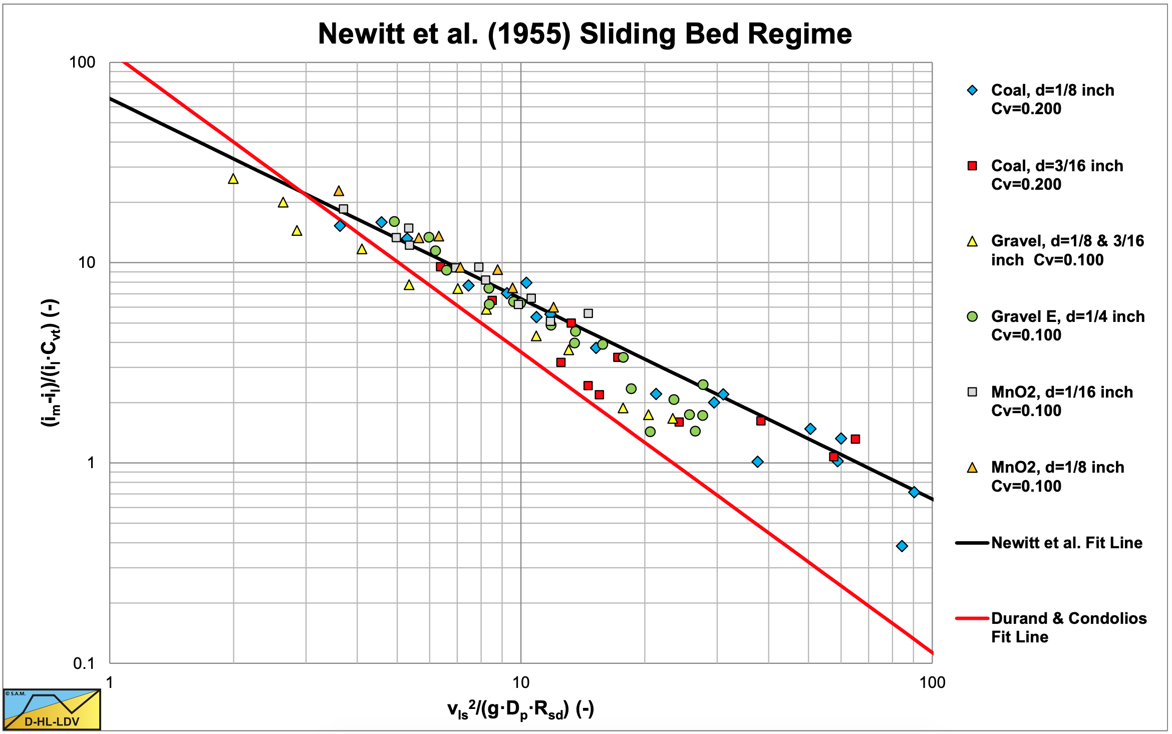
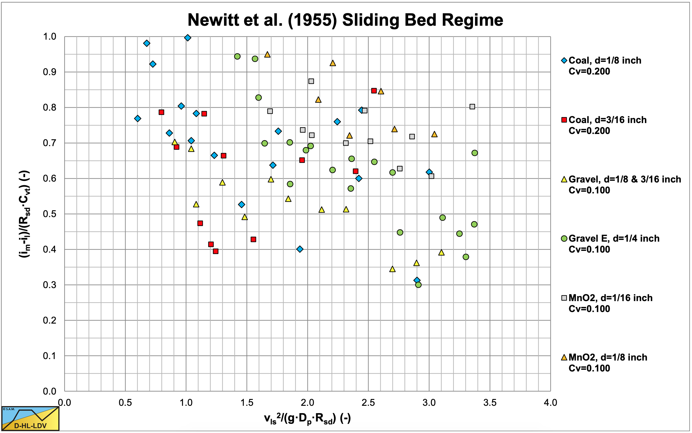
For the sliding bed regime Newitt et al. (1955) assumed that the weight of all the solids is transferred to the pipe bottom, resulting in a friction force, which is equal to the weight of the solids \(\ \rho_{\mathrm{l}} \cdot \mathrm{g} \cdot \mathrm{R}_{\mathrm{sd}} \cdot \mathrm{C}_{\mathrm{vt}}\) times a friction coefficient μ. They carried out experiments with gravel of 3.2-6.4 mm, coal of 3.2-4.8 mm (R_sd =0.4) and MnO2 of 1.6-3.2 mm (R_sd =3.1). Figure 6.5-2 and Figure 6.5-3 show the results of these experiments, Figure 6.5-3 with a new coordinate on the vertical axis (i_m − i_l ) / (R_sd ^. C_vt ) . The advantage of this parameter is that for a sliding bed it gives the friction coefficient μ_sf directly.

Below the Limit Deposit Velocity Newitt et al. (1955) found for a sliding bed:

\[\ \begin{array}{left}\Delta \mathrm{p}_{\mathrm{m}}=\Delta \mathrm{p}_{\mathrm{l}} \cdot\left(\mathrm{1}+\mathrm{K}_{2} \cdot\left(\mathrm{g} \cdot \mathrm{D}_{\mathrm{p}} \cdot \mathrm{R}_{\mathrm{s d}}\right) \cdot \mathrm{C}_{\mathrm{v} \mathrm{t}} \cdot\left(\frac{\mathrm{1}}{\mathrm{v}_{\mathrm{l s}}}\right)^{2}\right)\\
\mathrm{K}_{2}=\mathrm{6 6}\end{array}\]

Newitt et al. (1955) considered a sliding bed with a friction coefficient of μ_sf=0.8, but an analysis of the data points shows a decreasing tendency with increasing line speed. This matches the constant volumetric transport concentration model, which seems to be applied by Newitt et al. (1955). Friction coefficients of 0.35-0.7 have to be used to make the data points match the theory. The different materials have different friction coefficients. A better average of the friction coefficient would be μ_sf=0.66, matching a friction factor λ_l=0.02 and K₂=66.

Since Newitt et al. (1955) considered the solids effect to be the result of sliding friction, this solids effect should not depend on the viscous friction, although equation (6.5-3) implies this. In a D_p=1 inch pipe a friction coefficient of λ_l=0.02 is common, while in a D_p=1 m pipe a λ_l=0.01 would be expected. The difference is at least a factor 2.

In a large diameter pipe with much less liquid friction, the solids effect should be the same as in a small diameter pipe. In order to achieve this, equation (6.5-3) will be written in a more general form.

Figure 6.5-2: Correlation for large particles travelling as a sliding bed.

Figure 6.5-3: Large particles travelling in saltation or as a sliding bed.

Equation (6.5-3) in a more general form:

\[\ \begin{array}{left} \Delta \mathrm{p}_{\mathrm{m}}=\Delta \mathrm{p}_{\mathrm{l}} \cdot\left(\mathrm{1}+\left(\frac{\lambda_{\mathrm{l}} \cdot \mathrm{K}_{2}}{\mathrm{2}}\right) \cdot \frac{\mathrm{2} \cdot\left(\mathrm{g} \cdot \mathrm{D}_{\mathrm{p}} \cdot \mathrm{R}_{\mathrm{s} \mathrm{d}}\right)}{\lambda_{\mathrm{l}}} \cdot \mathrm{C}_{\mathrm{v t}} \cdot\left(\frac{\mathrm{1}}{\mathrm{v}_{\mathrm{ls}}}\right)^{2}\right)\\
\text { With : } \lambda_{1}=0.02 \text { and } \mathrm{K}_{2}=66 \text { this gives: }\\
\Delta \mathrm{p}_{\mathrm{m}}=\Delta \mathrm{p}_{\mathrm{l}} \cdot\left(\mathrm{1}+\mathrm{0 . 6 6} \cdot \frac{\mathrm{2} \cdot\left(\mathrm{g} \cdot \mathrm{D}_{\mathrm{p}} \cdot \mathrm{R}_{\mathrm{s} \mathrm{d}}\right)}{\lambda_{\mathrm{l}}} \cdot \mathrm{C}_{\mathrm{v t}} \cdot\left(\frac{\mathrm{1}}{\mathrm{v}_{\mathrm{l s}}}\right)^{2}\right)\\
\Delta \mathrm{p}_{\mathrm{m}}=\Delta \mathrm{p}_{\mathrm{l}}+\mathrm{0 . 6 6} \cdot \mathrm{g} \cdot \rho_{\mathrm{l}} \cdot \mathrm{R}_{\mathrm{s d}} \cdot \mathrm{C}_{\mathrm{vt}}\end{array}\]

Note that the 2^nd term between the brackets leads to a constant pressure loss independent of the line speed. The friction coefficient of 0.66 of course depends on the type of solids transported.

In the original graph of Newitt et al. (1955), Figure 6.5-2, the Durand & Condolios (1952) curve is incorrect, having the wrong slope (power). Most data points are below the Newitt et al. (1955) approximation for a sliding bed. A line with a steeper slope, so a higher power of the (1/v_ls) term would give a better fit. This matches the constant volumetric transport concentration behavior.

6.5.3 The Limit Deposit Velocity

The Limit Deposit Velocity is often defined as the velocity below which the first particles start to settle and a bed will be formed at the bottom of the pipe. Often this Limit Deposit Velocity is a bit smaller than the minimum velocity, which is at a pressure of 3 times the water resistance.

In Hydraulic Engineering it is assumed that particles stay in suspension when the so called friction velocity equals the settling velocity of the particles, giving:

\[\ \mathrm{u}_{*} \geq \mathrm{v}_{\mathrm{t}}\]

At the minimum resistance velocity this gives:

\[\ \mathrm{u}_{*}^{2}=\mathrm{3} \cdot \frac{\lambda_{\mathrm{l}}}{\mathrm{8}} \cdot \mathrm{v}_{\mathrm{l s}, \mathrm{ldv}}^{2}\]

Or (with λ=0.01):

\[\ \mathrm{v}_{\mathrm{l s}, \mathrm{ld v}}=\sqrt{\frac{\mathrm{8}}{\mathrm{3} \cdot \lambda_{\mathrm{l}}}} \cdot \mathrm{v}_{\mathrm{t}} \approx \mathrm{1 6 . 3 3} \cdot \mathrm{v}_{\mathrm{t}}\]

The limit Deposit Velocity found matches the findings of Newitt et al. (1955). Including the effect of hindered settling, this would result in a decreasing Limit Deposit Velocity with an increasing concentration, according to:

\[\ \mathrm{v}_{\mathrm{ls}, \mathrm{ldv}}=\sqrt{\frac{8}{3 \cdot \lambda_{1}}} \cdot \mathrm{v}_{\mathrm{t}} \cdot\left(1-\mathrm{C}_{\mathrm{vt}}\right)^{\beta} \approx 16.33 \cdot \mathrm{v}_{\mathrm{t}} \cdot\left(1-\mathrm{C}_{\mathrm{vt}}\right)^{\beta}\]

Newitt et al. (1955) used the following simple equation for the Limit Deposit Velocity:

\[\ \begin{array}{left} \frac{\mathrm{i}_{\mathrm{m}}-\mathrm{i}_{\mathrm{l}}}{\mathrm{i}_{\mathrm{l}} \cdot \mathrm{C}_{\mathrm{vt}}}=\mathrm{1 1 0 0} \cdot \frac{\mathrm{g} \cdot \mathrm{R}_{\mathrm{s d}} \cdot \mathrm{D}_{\mathrm{p}}}{\mathrm{v}_{\mathrm{l} \mathrm{s}, \mathrm{l d v}}^{\mathrm{2}}} \cdot \frac{\mathrm{v}_{\mathrm{t}}}{\mathrm{v}_{\mathrm{l} \mathrm{s}, \mathrm{l d v}}}=\mathrm{6 6} \cdot \frac{\mathrm{g} \cdot \mathrm{R}_{\mathrm{s d}} \cdot \mathrm{D}_{\mathrm{p}}}{\mathrm{v}_{\mathrm{l s}, \mathrm{l d v}}^{2}}\\
\Rightarrow \mathrm{v}_{\mathrm{l s}, \mathrm{l d v}}=\mathrm{1 6 . 6 7} \cdot \mathrm{v}_{\mathrm{t}}\end{array}\]

Newitt et al. (1955) assume that the transition between a sliding bed/saltation on one hand and a stationary bed on the other hand follow the well-known Durand & Condolios (1952) equation:

\[\ \mathrm{v}_{\mathrm{l} \mathrm{s}, \mathrm{l d v}}=\mathrm{F}_{\mathrm{L}} \cdot \sqrt{\mathrm{2} \cdot \mathrm{g} \cdot \mathrm{D}_{\mathrm{p}} \cdot \mathrm{R}_{\mathrm{s d}}}\]

The factor F_L can be found in the graph published by Durand & Condolios (1952) or by using equation (6.4-20). Newitt et al. (1955) used the graph of Durand (1953) with the factor F_L=1.34 for large particles.

6.5.4 The Transition Heterogeneous vs. (Pseudo) Homogeneous Transport

Newitt et al. (1955) found that the relative excess hydraulic gradient for (pseudo) homogeneous transport is not exactly the water resistance with the mixture density substituted for the water (liquid) density, but about 60% of the extra resistance, giving:

\[\ \begin{array}{left}\frac{\mathrm{i}_{\mathrm{m}}-\mathrm{i}_{\mathrm{l}}}{\mathrm{i}_{\mathrm{l}} \cdot \mathrm{C}_{\mathrm{v t}}}=\mathrm{0 . 6} \cdot \mathrm{R}_{\mathrm{s d}}\\
\frac{\mathrm{i}_{\mathrm{m}}-\mathrm{i}_{\mathrm{l}}}{\mathrm{i}_{\mathrm{l}} \cdot \mathrm{C}_{\mathrm{v t}}}=\mathrm{1 1 0 0} \cdot \frac{\mathrm{g} \cdot \mathrm{R}_{\mathrm{s d}} \cdot \mathrm{D}_{\mathrm{p}}}{\mathrm{v}_{\mathrm{l} \mathrm{s}, \mathrm{ld} \mathrm{v}}^{2}} \cdot \frac{\mathrm{v}_{\mathrm{t}}}{\mathrm{v}_{\mathrm{l s}, \mathrm{l d v}}}=\mathrm{0 . 6} \cdot \mathrm{R}_{\mathrm{s d}}\\
\Rightarrow \mathrm{v}_{\mathrm{l s}, \mathrm{h}=\mathrm{h}}=\sqrt[3]{\mathrm{1 8 3 3} \cdot \mathrm{g} \cdot \mathrm{D}_{\mathrm{p}} \cdot \mathrm{v}_{\mathrm{t}}}\end{array}\]

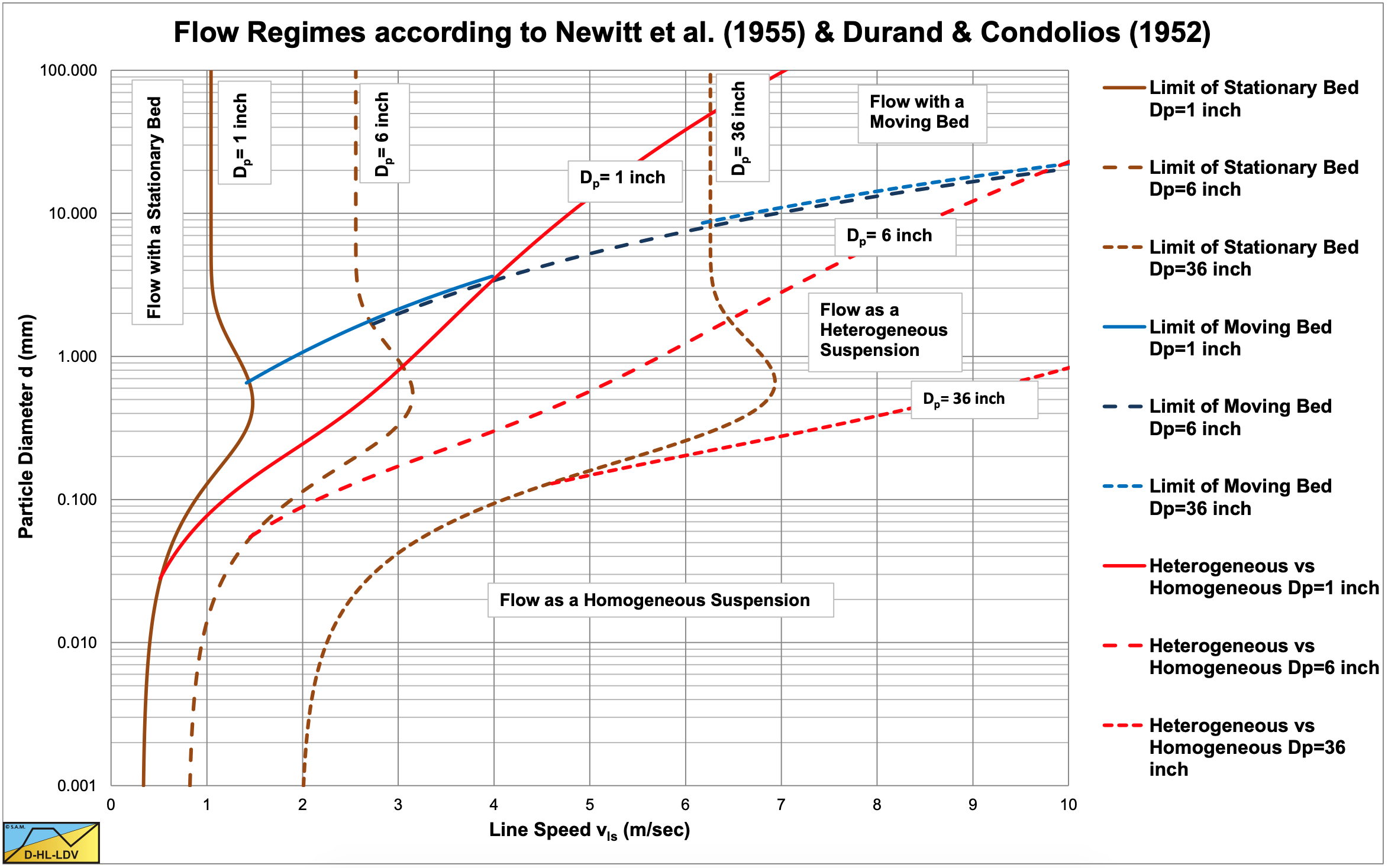
6.5.5 Regime Diagrams

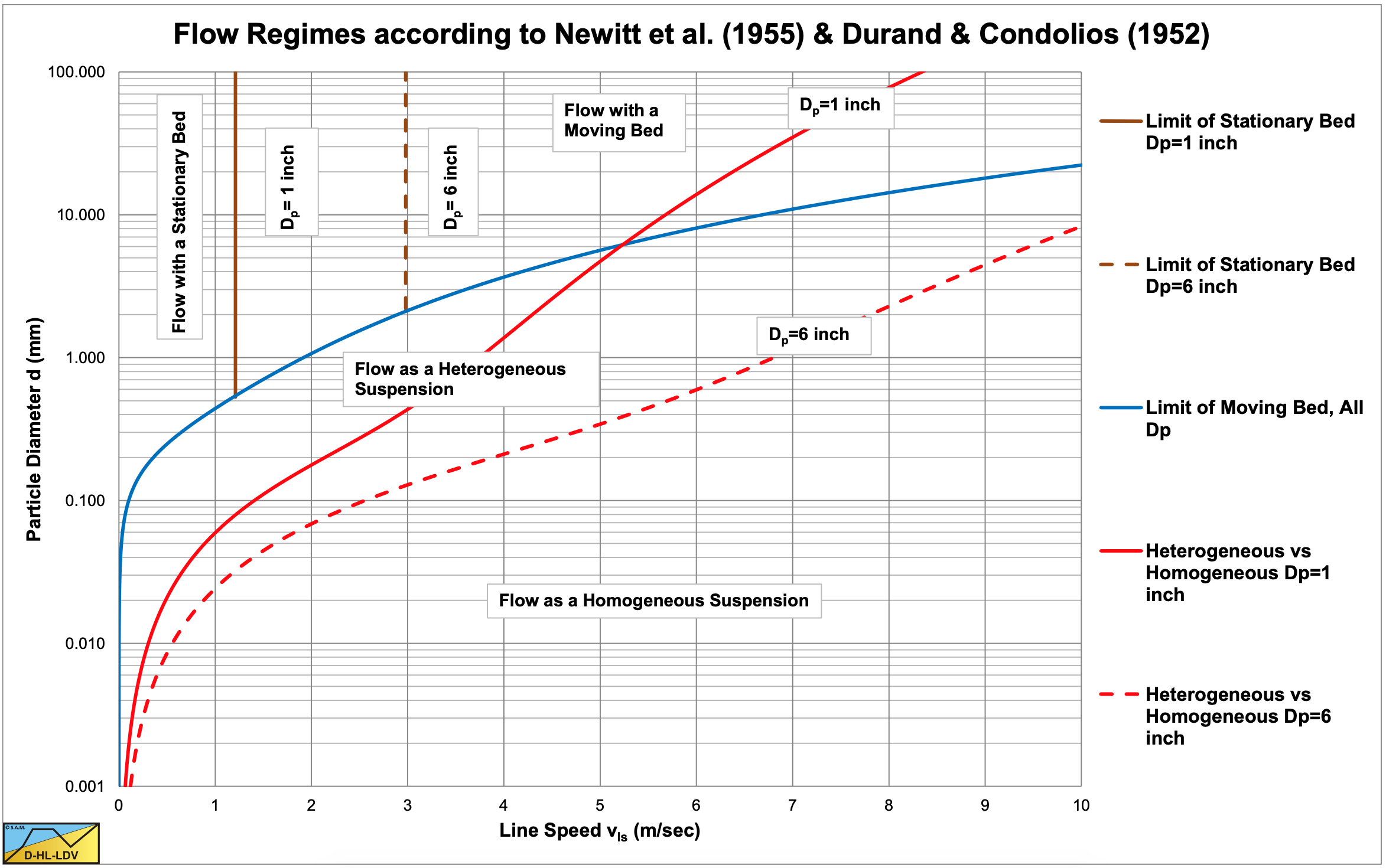
Based on the different transition velocities of Newitt et al. (1955) and the equation for the terminal settling velocity of Zanke (1977), the regime diagram of Newitt et al. (1955) has been reconstructed, see Figure 6.5-4. Now there are 3 issues regarding the equations of Newitt et al. (1955). The first issue is the issue of the error with the FL graph of Durand & Condolios (1952). The value for large particles should not be 1.34, but about 1.05 and corrected by a factor of 1.1 according to Gibert (1960). The second issue is that it is the question whether for homogeneous transport 60% of the solids weight should be applied, or the full 100%. Here 100% is applied. The third issue is the construction of the regime graph. The curves found by applying the equations, do not exactly match the curves of Newitt et al. (1955), but then in 1955 computers were not yet available. It should be noted that these regime diagrams do not incorporate the influence of the volumetric concentration. The regime diagrams of Newitt et al. (1955) however give a good impression of the different regimes and the transitions between the different regimes.

• For very small particles there will be a transition from a stationary bed to homogeneous flow directly.
• For small particles there will be a transition from a stationary bed to heterogeneous flow to homogeneous flow. For medium sized particles there will be a transition from a stationary bed to a moving bed to heterogeneous flow to homogeneous flow.
• For very large particles there will be a transition from a stationary bed to a moving bed to homogeneous flow directly.

Of course, this depends on the pipe diameter and the concentration. Especially the pipe diameter is playing a very big role in the location of the different transition lines. Figure 6.5-5 shows the regime diagram based on the equations derived here.

Figure 6.5-4: Flow regimes according to Newitt et al. (1955).

Figure 6.5-5: Flow regimes according to Durand & Condolios (1952) and Newitt et al. (1955), modified. (Captions for the 36 inch pipe diameter, C_v=0.15).

6.5.6 Experiments

Figure 6.5-6: The hydraulic gradient sand B.

Figure 6.5-7: The relative excess hydraulic gradient Sand B.

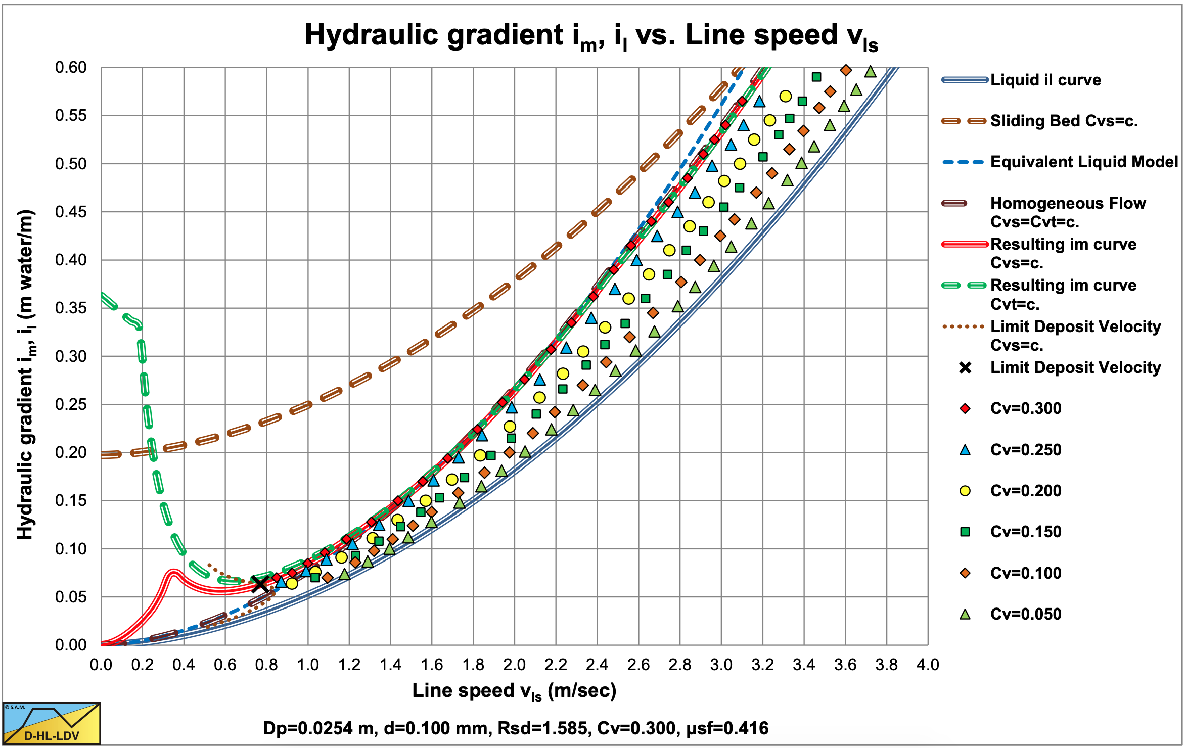
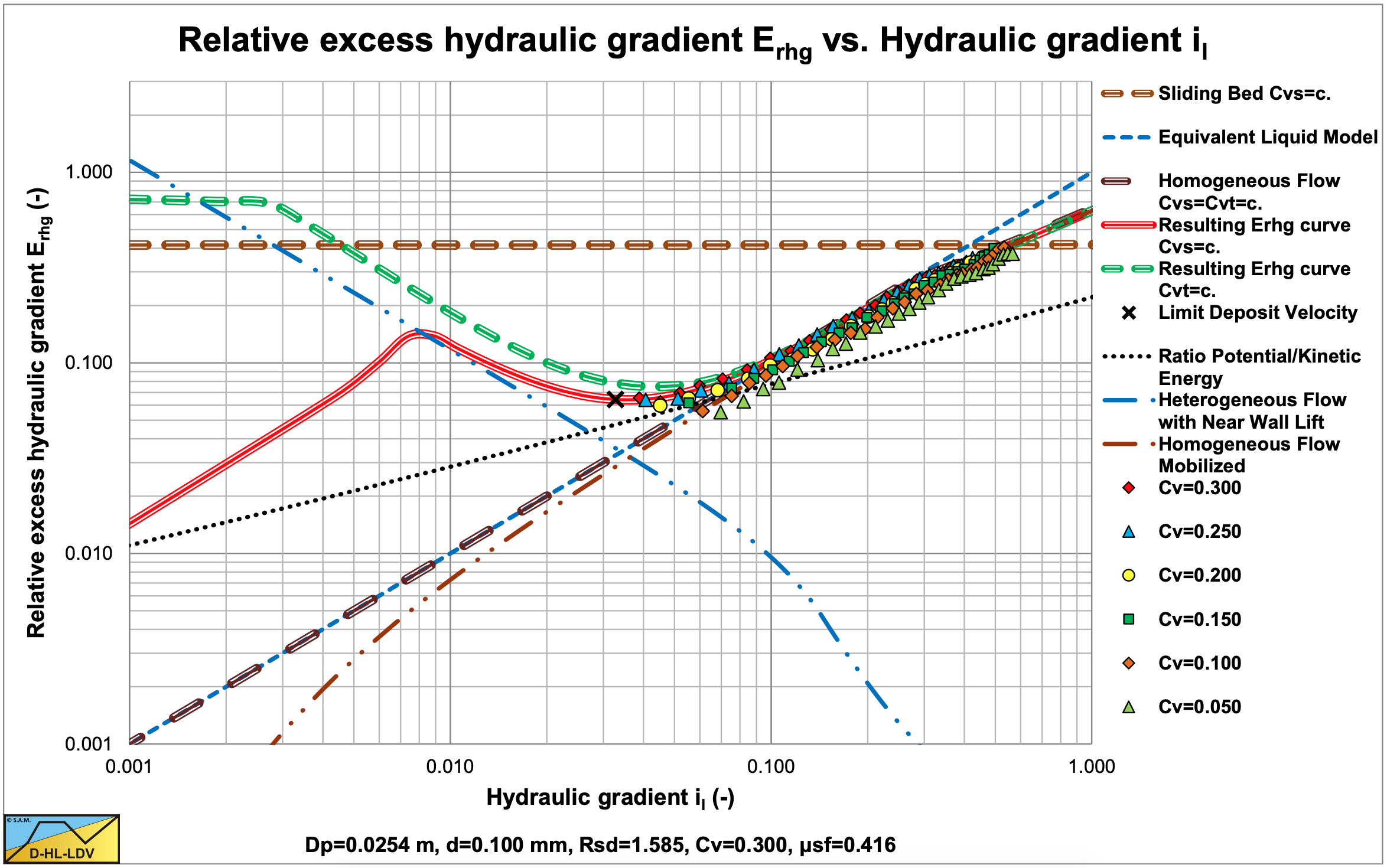
Figure 6.5-6 and Figure 6.5-7 show the digitized fit lines for sand B in the hydraulic gradient versus line speed graph and the relative excess hydraulic gradient versus liquid hydraulic gradient graph. Sand B behaves according to the Equivalent Liquid Model.

Figure 6.5-8: The hydraulic gradient sand C.

Figure 6.5-9: The relative excess hydraulic gradient Sand C.

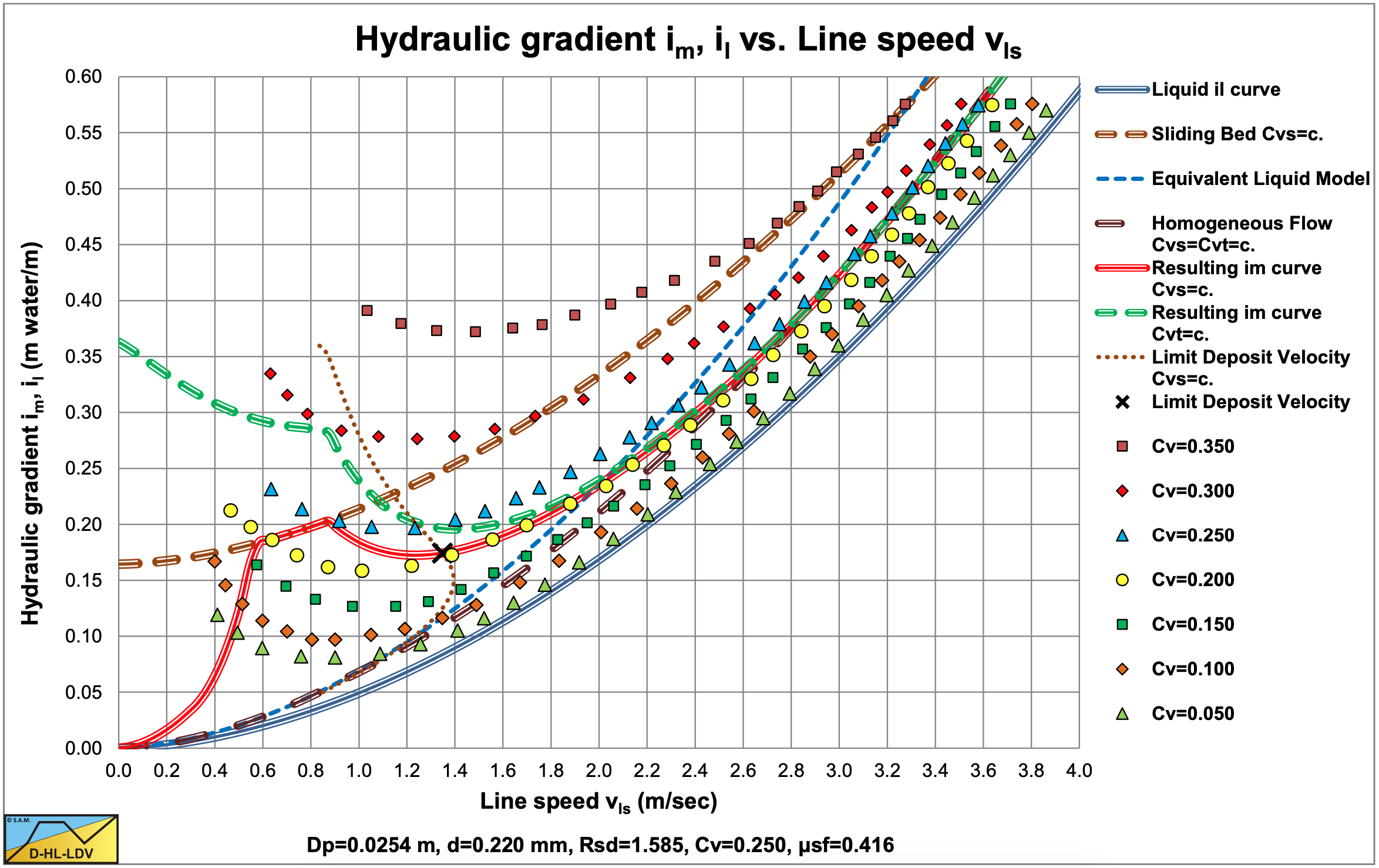
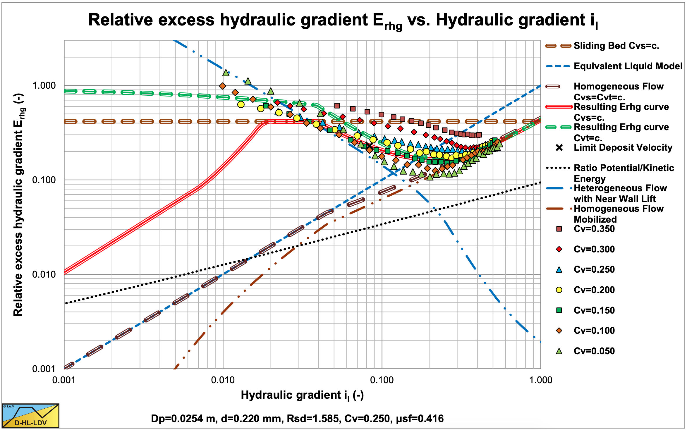
Figure 6.5-8 and Figure 6.5-9 show the digitized fit lines for sand B in the hydraulic gradient versus line speed graph and the relative excess hydraulic gradient versus liquid hydraulic gradient graph. Sand C behaves according to the sliding bed regimes at low lines speeds, the heterogeneous flow regime at medium line speeds and the homogeneous flow regime at high line speeds. Up to concentrations of 25% it matches the heterogeneous- homogeneous behavior. The concentrations of 30% and 35% give higher values, possibly due to sliding flow behavior.

Figure 6.5-10: The hydraulic gradient sand D.

Figure 6.5-11: The relative excess hydraulic gradient Sand D.

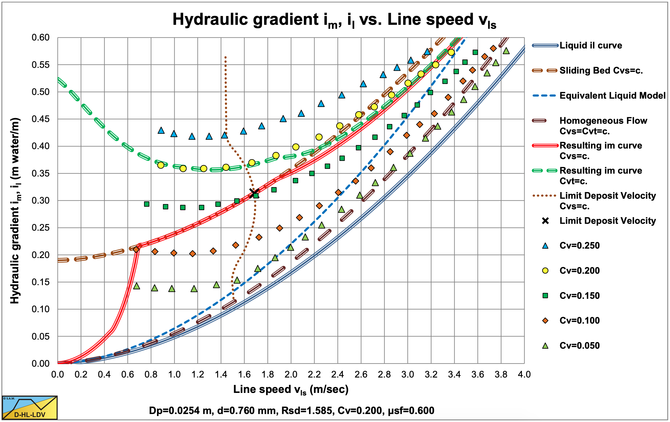
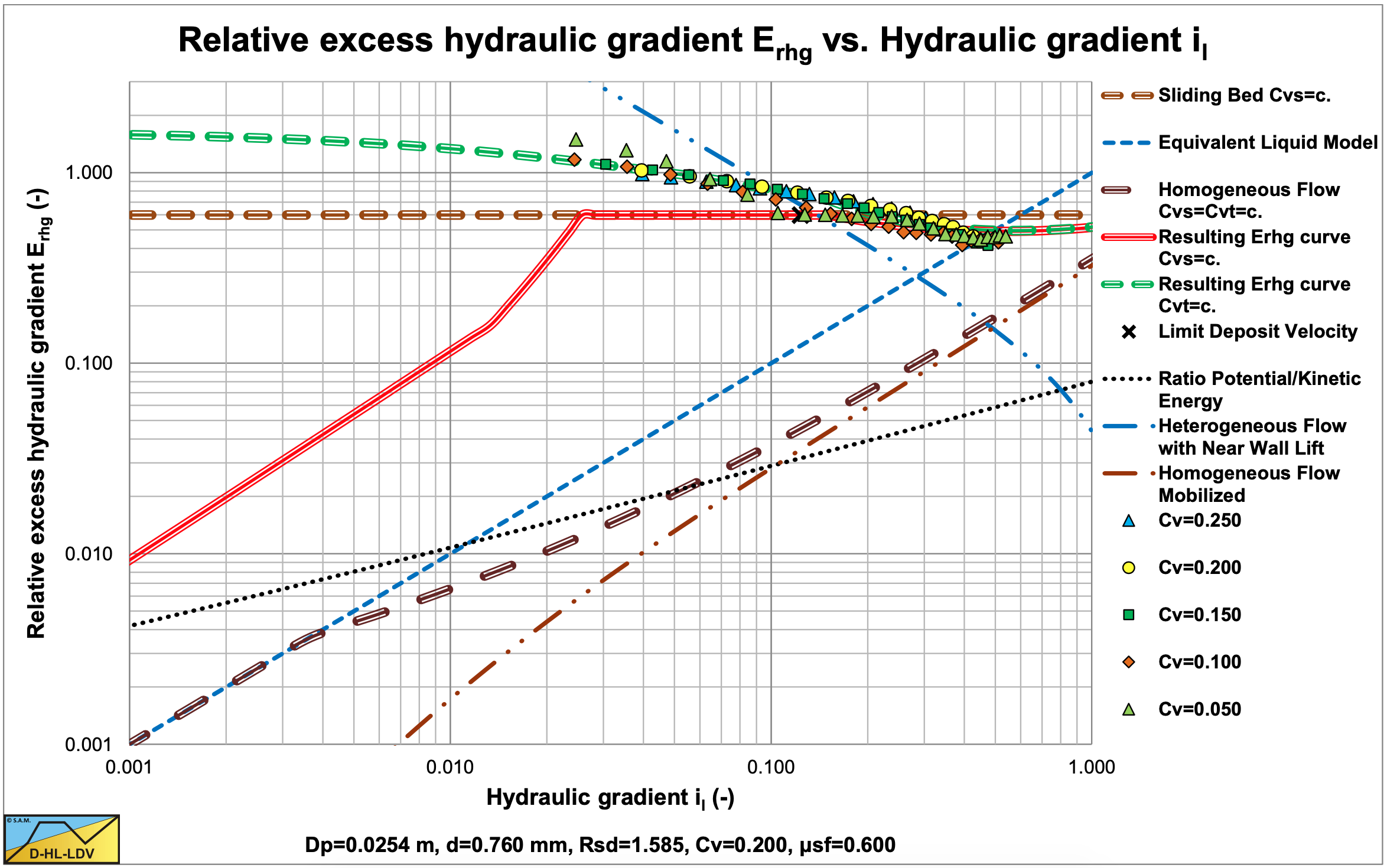
Figure 6.5-10 and Figure 6.5-11 show the digitized fit lines for sand B in the hydraulic gradient versus line speed graph and the relative excess hydraulic gradient versus liquid hydraulic gradient graph. Sand D behaves according to the sliding flow regime, a mix of heterogeneous and sliding bed behavior.

Figure 6.5-12: The hydraulic gradient sand E.

Figure 6.5-13: The relative excess hydraulic gradient Sand E.

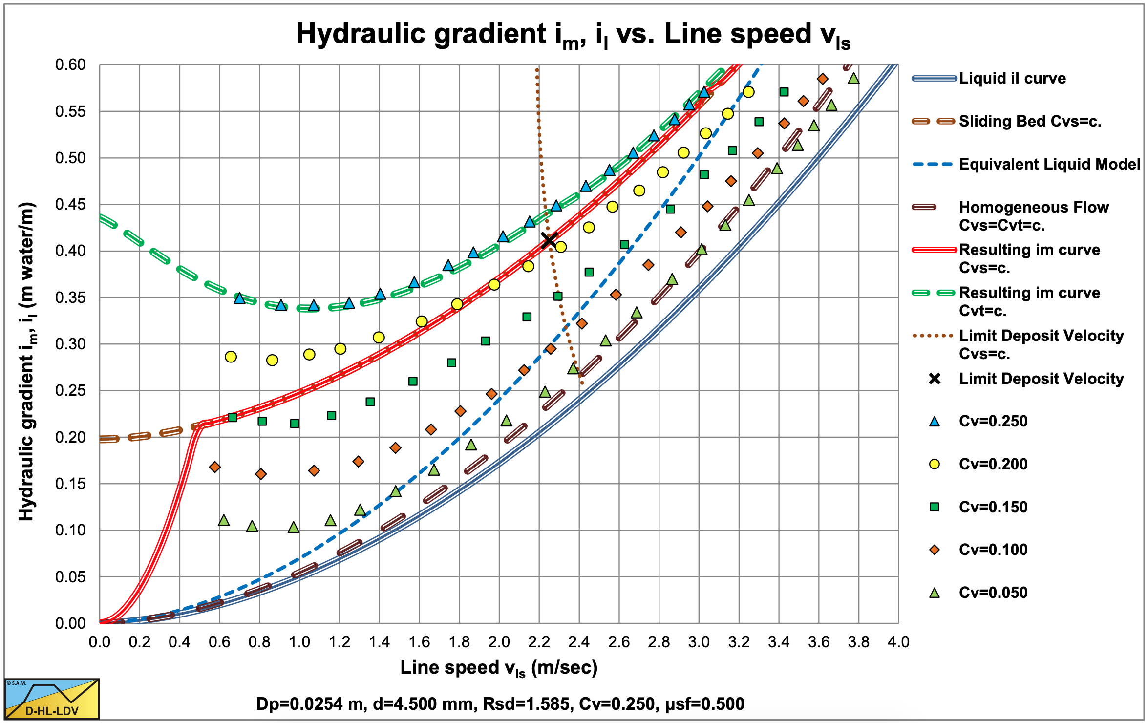
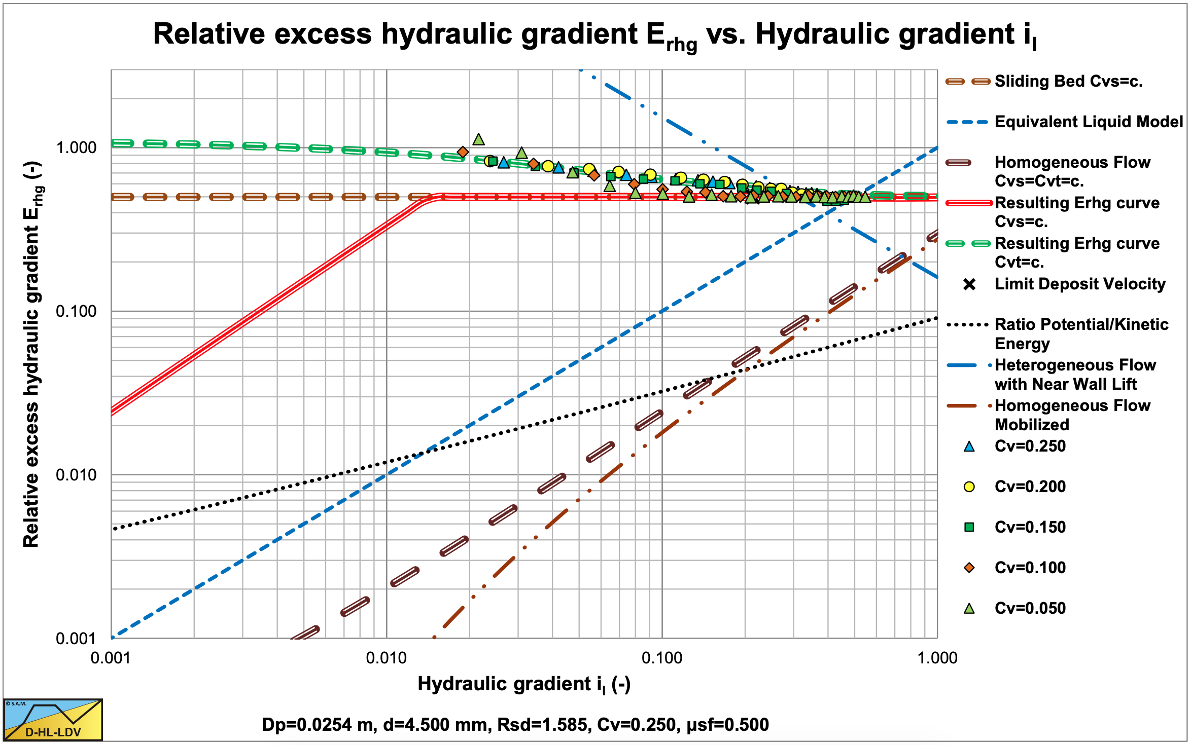
Figure 6.5-12 and Figure 6.5-13 show the digitized fit lines for sand B in the hydraulic gradient versus line speed graph and the relative excess hydraulic gradient versus liquid hydraulic gradient graph. Sand E (fine gravel) behaves according to the sliding bed flow regime.

6.5.7 Vertical Pipes

Newitt et al. (1961) investigated the hydraulic gradient of different solids in vertical pipes of 0.0254 and 0.0508 m diameter ( 1 and 2 inch pipes). They used sands (density 2.59-2.64 ton/m³) with diameters of 0.1, 0.19, 0.71 and 1.27 mm, pebbles (density 2.59 ton/m³) of 3.8 mm, Zircon (density 4.56 ton/m³) of 0.109 mm, Manganese dioxide (density 4.2 ton/m3) of 1.37 mm and Perspex (density 1.19 ton/m3) of 1.2 mm.

3 cases were considered:

1. Very small particles.
2. Medium sized particles.
3. Large particles.

Where the definitions of small, medium and large depend on the pipe diameter and the solids density.

6.5.7.1 Some Theoretical Considerations

The mass balance of the solids flow gives:

\[\ \mathrm{A}_{\mathrm{p}} \cdot \mathrm{C}_{\mathrm{v t}} \cdot \mathrm{v}_{\mathrm{l} \mathrm{s}} \cdot \mathrm{\rho}_{\mathrm{s}}=\mathrm{A}_{\mathrm{p}} \cdot \mathrm{C}_{\mathrm{v s}} \cdot \mathrm{v}_{\mathrm{s}} \cdot \mathrm{\rho}_{\mathrm{s}}=\mathrm{A}_{\mathrm{p}} \cdot \mathrm{C}_{\mathrm{v s}} \cdot\left(\mathrm{v}_{\mathrm{l}}-\mathrm{v}_{\mathrm{t h}}\right) \cdot \mathrm{\rho}_{\mathrm{s}}\]

Or:

\[\ \mathrm{C}_{\mathrm{v t}} \cdot \mathrm{v}_{\mathrm{l s}}=\mathrm{C}_{\mathrm{v s}} \cdot \mathrm{v}_{\mathrm{s}}=\mathrm{C}_{\mathrm{v s}} \cdot\left(\mathrm{v}_{\mathrm{l}}-\mathrm{v}_{\mathrm{t h}}\right)\]

In this mass balance it is assumed that the particles (solids) have a velocity v_s smaller than the cross sectional averaged line speed v_ls and the liquid (water) has a larger velocity v_l. In the original publication transport concentration is used for spatial concentration. Here spatial volumetric concentration C_vs and delivered or transport volumetric concentration C_vt are used.

The mass balance of the liquid (water) gives:

\[\ \mathrm{A}_{\mathrm{p}} \cdot\left(\mathrm{1}-\mathrm{C}_{\mathrm{v t}}\right) \cdot \mathrm{v}_{\mathrm{l s}} \cdot \mathrm{\rho}_{\mathrm{l}}=\mathrm{A}_{\mathrm{p}} \cdot\left(\mathrm{1}-\mathrm{C}_{\mathrm{v s}}\right) \cdot \mathrm{v}_{\mathrm{l}} \cdot \mathrm{\rho}_{\mathrm{l}}\]

Or:

\[\ \mathrm{\left(1-C_{v t}\right) \cdot v_{l s}=\left(1-C_{v s}\right) \cdot v_{1}}\]

This gives for the liquid velocity v_l, assuming the terminal hindered settling velocity v_th is known (ascending pipe: a positive terminal hindered settling velocity, descending pipe: a negative terminal hindered settling velocity):

\[\ \mathrm{v}_{\mathrm{l}}=\mathrm{v}_{\mathrm{l} \mathrm{s}}+\mathrm{C}_{\mathrm{v s}} \cdot \mathrm{v}_{\mathrm{t h}}\]

If the spatial volumetric concentration is known, the delivered or transport volumetric concentration can be determined according to:

\[\ \mathrm{C}_{\mathrm{v t}}=\mathrm{C}_{\mathrm{v s}} \cdot\left(\mathrm{1}-\frac{\mathrm{v}_{\mathrm{t h}}}{\mathrm{v}_{\mathrm{l s}}}\right)+\mathrm{C}_{\mathrm{v s}}^{2} \cdot \frac{\mathrm{v}_{\mathrm{t h}}}{\mathrm{v}_{\mathrm{l s}}}\]

If the delivered volumetric concentration is known, the spatial volumetric concentration can be determined according to:

\[\ \mathrm{C}_{\mathrm{v s}}=-\frac{\mathrm{1}}{2} \cdot\left(\frac{\mathrm{v}_{\mathrm{l s}}}{\mathrm{v}_{\mathrm{t h}}}-\mathrm{1}\right)+\frac{\mathrm{1}}{2} \cdot \sqrt{\left(\frac{\mathrm{v}_{\mathrm{l s}}}{\mathrm{v}_{\mathrm{t h}}}-\mathrm{1}\right)^{2}+\mathrm{4} \cdot \mathrm{C}_{\mathrm{v t}} \cdot \frac{\mathrm{v}_{\mathrm{l s}}}{\mathrm{v}_{\mathrm{t h}}}}\]

6.5.7.2 Additions to Newitt et al. (1961)

Now considering the vertical transport over a period of time Δt. The mixture as a whole has travelled a vertical distance ΔH=v_ls·Δt. The mass flux Q_m,t and the mass transport ΔM_t are now:

\[\ \begin{array}{}
\mathrm{Q_{m,t} =A_p \cdot C_{vt} \cdot v_{ls} \cdot \rho_{s} + A_p \cdot (1-C_{vt})\cdot v_{ls} \cdot \rho_l}\\
\mathrm{\Delta M_t =Q_{m,t}\cdot \Delta t=A_p \cdot C_{vt}\cdot v_{ls}\cdot \rho_s \cdot \Delta t + A_p \cdot (1-C_{vt})\cdot v_{ls} \cdot \rho_l \cdot \Delta t }\\
\mathrm{\Delta M_t=A_p \cdot v_{ls}\cdot \Delta t \cdot (C_{vt}\cdot \rho_s +(1-C_{vt})\cdot \rho_l)=\Delta V \cdot \rho_{m,t} }
\end{array}\]

The potential energy ΔE_p,t gained by the transported mixture is now:

\[\ \Delta \mathrm{E}_{\mathrm{p}, \mathrm{t}}=\Delta \mathrm{M}_{\mathrm{t}} \cdot \mathrm{g} \cdot \Delta \mathrm{H}=\mathrm{A}_{\mathrm{p}} \cdot \mathrm{v}_{\mathrm{l s}} \cdot \Delta \mathrm{t} \cdot\left(\mathrm{C}_{\mathrm{v} \mathrm{t}} \cdot \rho_{\mathrm{s}}+\left(\mathrm{1}-\mathrm{C}_{\mathrm{v} \mathrm{t}}\right) \cdot \rho_{\mathrm{l}}\right) \cdot \mathrm{g} \cdot \Delta \mathrm{H}=\Delta \mathrm{V} \cdot \rho_{\mathrm{m}, \mathrm{t}} \cdot \mathrm{g} \cdot \Delta \mathrm{H}\]

The work carried out however is based on the spatial concentration in the pipe, giving:

\[\ \Delta \mathrm{E}_{\mathrm{p}, \mathrm{s}}=\Delta \mathrm{M}_{\mathrm{s}} \cdot \mathrm{g} \cdot \Delta \mathrm{H}=\mathrm{A}_{\mathrm{p}} \cdot \mathrm{v}_{\mathrm{l} \mathrm{s}} \cdot \Delta \mathrm{t} \cdot\left(\mathrm{C}_{\mathrm{v s}} \cdot \rho_{\mathrm{s}}+\left(\mathrm{1}-\mathrm{C}_{\mathrm{v s}}\right) \cdot \rho_{\mathrm{l}}\right) \cdot \mathrm{g} \cdot \Delta \mathrm{H}=\Delta \mathrm{V} \cdot \rho_{\mathrm{m}, \mathrm{s}} \cdot \mathrm{g} \cdot \Delta \mathrm{H}\]

This follows from the fact that this work equals the required pressure Δp times the mixture flow Q_v times the period of time Δt. The required pressure is the weight ΔM_s·g of the column of mixture in the pipe with height ΔH divided by the cross section of the pipe A_p.

\[\ \Delta \mathrm{p}=\frac{\Delta \mathrm{M}_{\mathrm{s}} \cdot \mathrm{g}}{\mathrm{A}_{\mathrm{p}}}=\frac{\mathrm{A}_{\mathrm{p}} \cdot \mathrm{v}_{\mathrm{l s}} \cdot \Delta \mathrm{t} \cdot\left(\mathrm{C}_{\mathrm{v s}} \cdot \mathrm{\rho}_{\mathrm{s}}+\left(\mathrm{1}-\mathrm{C}_{\mathrm{v s}}\right) \cdot \rho_{\mathrm{l}}\right) \cdot \mathrm{g}}{\mathrm{A}_{\mathrm{p}}}=\frac{\Delta \mathrm{V} \cdot \rho_{\mathrm{m}, \mathrm{s}} \cdot \mathrm{g}}{\mathrm{A}_{\mathrm{p}}}\]

So the work required is now:

\[\ \begin{aligned} \Delta \mathrm{E}_{\mathrm{p}, \mathrm{s}} &=\Delta \mathrm{p} \cdot \mathrm{Q}_{\mathrm{v}} \cdot \Delta \mathrm{t}=\Delta \mathrm{p} \cdot \mathrm{v}_{\mathrm{l} \mathrm{s}} \cdot \mathrm{A}_{\mathrm{p}} \cdot \Delta \mathrm{t}=\Delta \mathrm{p} \cdot \mathrm{A}_{\mathrm{p}} \cdot \Delta \mathrm{H} \\ &=\frac{\mathrm{A}_{\mathrm{p}} \cdot \mathrm{v}_{\mathrm{l} \mathrm{s}} \cdot \Delta \mathrm{t} \cdot\left(\mathrm{C}_{\mathrm{v} \mathrm{s}} \cdot \rho_{\mathrm{s}}+\left(\mathrm{1}-\mathrm{C}_{\mathrm{v} \mathrm{s}}\right) \cdot \rho_{\mathrm{l}}\right) \cdot \mathrm{g}}{\mathrm{A}_{\mathrm{p}}}\\&=\mathrm{A}_{\mathrm{p}} \cdot \mathrm{v}_{\mathrm{l} \mathrm{s}} \cdot \Delta \mathrm{t} \cdot\left(\mathrm{C}_{\mathrm{v} \mathrm{s}} \cdot \rho_{\mathrm{s}}+\left(\mathrm{1}-\mathrm{C}_{\mathrm{v} \mathrm{s}}\right) \cdot \rho_{\mathrm{l}}\right) \cdot \mathrm{g} \cdot \Delta \mathrm{H} \end{aligned}\]

The difference between the work carried out and the potential energy gained by the mixture is:

\[\ \begin{aligned} \Delta \mathrm{E}_{\mathrm{p}, \mathrm{s}}-\Delta \mathrm{E}_{\mathrm{p}, \mathrm{t}} &=\mathrm{A}_{\mathrm{p}} \cdot \mathrm{v}_{\mathrm{l s}} \cdot \Delta \mathrm{t} \cdot\left(\mathrm{C}_{\mathrm{v} \mathrm{s}} \cdot \rho_{\mathrm{s}}+\left(\mathrm{1}-\mathrm{C}_{\mathrm{v} \mathrm{s}}\right) \cdot \rho_{\mathrm{l}}\right) \cdot \mathrm{g} \cdot \mathrm{\Delta} \mathrm{H} \\ &-\mathrm{A}_{\mathrm{p}} \cdot \mathrm{v}_{\mathrm{l s}} \cdot \Delta \mathrm{t} \cdot\left(\mathrm{C}_{\mathrm{v t}} \cdot \rho_{\mathrm{s}}+\left(\mathrm{1}-\mathrm{C}_{\mathrm{v} \mathrm{t}}\right) \cdot \rho_{\mathrm{l}}\right) \cdot \mathrm{g} \cdot \mathrm{\Delta} \mathrm{H} \\ &=\mathrm{A}_{\mathrm{p}} \cdot \mathrm{v}_{\mathrm{l} \mathrm{s}} \cdot \Delta \mathrm{t} \cdot \mathrm{g} \cdot \Delta \mathrm{H} \cdot\left(\mathrm{C}_{\mathrm{v s}}-\mathrm{C}_{\mathrm{v} \mathrm{t}}\right) \cdot\left(\rho_{\mathrm{s}}-\rho_{\mathrm{l}}\right) \end{aligned}\]

Substituting the relation between spatial and delivered concentration gives for this difference:

\[\ \Delta \mathrm{E}_{\mathrm{p}, \mathrm{s}}-\Delta \mathrm{E}_{\mathrm{p}, \mathrm{t}}=\mathrm{A}_{\mathrm{p}} \cdot \mathrm{v}_{\mathrm{t h}} \cdot \Delta \mathrm{t} \cdot \mathrm{g} \cdot \Delta \mathrm{H} \cdot\left(\mathrm{C}_{\mathrm{v s}}-\mathrm{C}_{\mathrm{v s}}^{2}\right) \cdot\left(\rho_{\mathrm{s}}-\rho_{\mathrm{l}}\right)\]

This is the energy dissipated due to the viscous friction around the particles. This dissipated energy depends on the terminal hindered settling velocity and on the spatial concentration. The pressure required depends on the spatial concentration. For small particles with a small value of the terminal hindered settling velocity, the dissipated energy will also be small, however for large particles like gravel this will not be the case.

6.5.7.3 Correction on the Darcy Weisbach Friction Factor

The hydraulic gradient for pure liquid flow is:

\[\ \mathrm{i}_{\mathrm{l}}=\frac{\lambda_{1} \cdot \mathrm{v}_{\mathrm{ls} }^{2}}{2 \cdot \mathrm{g} \cdot \mathrm{D}_{\mathrm{p}}}\]

Since the liquid velocity is higher, depending on the spatial concentration and the terminal hindered settling velocity, the velocity in this equation should be replaced by the liquid velocity, assuming that the Darcy Weisbach friction factor hardly changes at high Reynolds numbers. This gives for the hydraulic gradient of a mixture in a vertical pipe, assuming the equivalent liquid model is valid:

\[\ \begin{array}{} \mathrm{i}_{\mathrm{m}}=\frac{\rho_{\mathrm{m}}}{\rho_{\mathrm{l}}} \cdot \frac{\lambda_{\mathrm{l}} \cdot\left(\mathrm{v}_{\mathrm{l} \mathrm{s}}+\mathrm{C}_{\mathrm{v s}} \cdot \mathrm{v}_{\mathrm{t h}}\right)^{2}}{2 \cdot \mathrm{g} \cdot \mathrm{D}_{\mathrm{p}}}=\frac{\rho_{\mathrm{m}}}{\rho_{\mathrm{l}}} \cdot \frac{\lambda_{\mathrm{l}} \cdot\left(\mathrm{v}_{\mathrm{l} \mathrm{s}}^{2}+\mathrm{2} \cdot \mathrm{C}_{\mathrm{v} \mathrm{s}} \cdot \mathrm{v}_{\mathrm{t h}} \cdot \mathrm{v}_{\mathrm{l} \mathrm{s}}+\mathrm{C}_{\mathrm{v} \mathrm{s}}^{2} \cdot \mathrm{v}_{\mathrm{t h}}^{2}\right)}{\mathrm{2} \cdot \mathrm{g} \cdot \mathrm{D}_{\mathrm{p}}}\\
\mathrm{i}_{\mathrm{m}} \approx \frac{\rho_{\mathrm{m}}}{\rho_{\mathrm{l}}} \cdot \frac{\lambda_{1} \cdot\left(\mathrm{v}_{\mathrm{l} \mathrm{s}}^{2}+\mathrm{2} \cdot \mathrm{C}_{\mathrm{v} \mathrm{s}} \cdot \mathrm{v}_{\mathrm{t h}} \cdot \mathrm{v}_{\mathrm{l s}}\right)}{\mathrm{2} \cdot \mathrm{g} \cdot \mathrm{D}_{\mathrm{p}}}=\frac{\rho_{\mathrm{m}}}{\rho_{\mathrm{l}}} \cdot \frac{\lambda_{1} \cdot \mathrm{v}_{\mathrm{ls}}^{2}}{\mathrm{2} \cdot \mathrm{g} \cdot \mathrm{D}_{\mathrm{p}}}+\frac{\rho_{\mathrm{m}}}{\rho_{\mathrm{l}}} \cdot \frac{\mathrm{2} \cdot \lambda_{1} \cdot \mathrm{C}_{\mathrm{v} \mathrm{s}} \cdot \mathrm{v}_{\mathrm{t h}} \cdot \mathrm{v}_{\mathrm{ls}}}{\mathrm{2} \cdot \mathrm{g} \cdot \mathrm{D}_{\mathrm{p}}}\end{array}\]

Since normally the spatial concentration will have a value from 0-0.4, the terminal settling velocity has a value of 0.4 m/s for a 10 mm particle and the terminal hindered settling velocity is always smaller, the quadratic term of spatial concentration times terminal hindered settling velocity is negligible for line speeds above 1 m/s. With a line speed of 1 m/s, a spatial concentration of 0.4 and a terminal settling velocity of 0.4 m/s, the second term on the right hand side 30% of the first term, which is significant. Using the terminal hindered settling velocity in this case of 0.11 m/s gives about 8%, which is still significant. For small particles the second term on the right hand side can be neglected.

6.5.7.4 The Magnus Effect

If a particle is situated near the wall of a vertical conveying pipe in which the velocity gradient is steep, the particle will be subjected to forces which tend to cause it to rotate and to move towards the axis of the pipe. Both turbulent lift caused by a velocity different over the particle in a pipe radial direction and Magnus lift due to the rotation of the particle will cause such a lift force and push particles away from the pipe wall. This way a particle poor or particles free viscous sub layer is created.

6.5.7.5 Experimental Results

Newitt et al. (1961) found that for small particles the hydraulic gradient follows the equivalent liquid model.

\[\ \mathrm{i}_{\mathrm{m}}=\frac{\rho_{\mathrm{m}}}{\rho_{\mathrm{l}}} \cdot \frac{\lambda_{\mathrm{l}} \cdot \mathrm{v}_{\mathrm{ls}}^{2}}{2 \cdot \mathrm{g} \cdot \mathrm{D}_{\mathrm{p}}}\]

The experiments were carried out with sand with d=0.1 mm, sand with d=0.19 mm and Zircon sand with d=0.109 mm.

Sand with d=0.71 mm and Perspex with d=1.2 mm show hydraulic gradients identical to pure liquid with the same average line speeds.

Pebbles with d=4.2 mm and Manganese dioxide with d=1.37 mm show an excess hydraulic gradient (solids effect) at low line speeds, decreasing to almost zero at high line speeds.

Newitt et al. (1961) found an empirical relation for this behavior, giving:

\[\ \frac{\mathrm{i}_{\mathrm{m}}-\mathrm{i}_{\mathrm{l}}}{\mathrm{C}_{\mathrm{v} \mathrm{t}} \cdot \mathrm{i}_{\mathrm{l}}}=\mathrm{0 . 0 0 3 7} \cdot\left(\frac{\mathrm{g} \cdot \mathrm{D}_{\mathrm{p}}}{\mathrm{v}_{\mathrm{l s}}^{\mathrm{2}}}\right)^{1 / 2} \cdot\left(\frac{\mathrm{D}_{\mathrm{p}}}{\mathrm{d}}\right) \cdot\left(\frac{\rho_{\mathrm{s}}}{\rho_{\mathrm{l}}}\right)^{2}\]

6.5.7.6 Discussion & Conclusions

Based on the equivalent liquid model this would give:

\[\ \frac{\mathrm{i}_{\mathrm{m}}-\mathrm{i}_{\mathrm{l}}}{\mathrm{C}_{\mathrm{vt}} \cdot \mathrm{i}_{\mathrm{l}}}=\frac{\frac{\rho_{\mathrm{m}}}{\rho_{\mathrm{l}}} \cdot \frac{\lambda_{\mathrm{l}} \cdot \mathrm{v}_{\mathrm{ls}}^{2}}{2 \cdot \mathrm{g} \cdot \mathrm{D}_{\mathrm{p}}}-\frac{\lambda_{\mathrm{l}} \cdot \mathrm{v}_{\mathrm{ls}}^{2}}{2 \cdot \mathrm{g} \cdot \mathrm{D}_{\mathrm{p}}}}{\mathrm{C}_{\mathrm{vt}} \cdot \frac{\lambda_{1} \cdot \mathrm{v}_{\mathrm{ls}}^{2}}{2 \cdot \mathrm{g} \cdot \mathrm{D}_{\mathrm{p}}}}=\frac{\frac{\rho_{\mathrm{m}}}{\rho_{\mathrm{l}}}-1}{\mathrm{C}_{\mathrm{vt}}}=\frac{\mathrm{R}_{\mathrm{sd}} \cdot \mathrm{C}_{\mathrm{vs}}}{\mathrm{C}_{\mathrm{vt}}} \approx \mathrm{R}_{\mathrm{sd}}\]

So for small particles, where the spatial and delivered concentration do not differ too much, this is equal to the relative submerged density R_sd. This means that the maximum value of the Newitt et al. (1961) equation is the relative submerged density or a slightly higher value in case of medium to large particles. Newitt et al. (1961) do not mention this limitation.

The use of dimensionless numbers containing the pipe diameter is questionable, since only 0.0254 m (1 inch) and 0.0508 m (2 inch) pipes are used in the research and only results with the 0.0254 m (1 inch) pipe are shown in the publication. Since the purpose of the equation is to quantify the effect of a particle free or poor viscous sub-layer due to near wall lift, the equation should be based on near wall phenomena. If the particle diameter is larger than the thickness of the viscous sub-layer, the concentration in the viscous sub-layer will be smaller than the cross sectional averaged concentration. Although this concentration effect is not linear with the particle diameter, as a first attempt a linear relation is used. The ratio of the thickness of the viscous sub-layer to the particle diameter is:

\[\ \frac{\mathrm{\delta_{v}}}{\mathrm{d}}=\frac{11.6 \cdot \frac{v_{\mathrm{l}}}{\mathrm{u}_{*}}}{\mathrm{d}}=\frac{11.6 \cdot v_{\mathrm{l}}}{\sqrt{\lambda_{1} / 8} \cdot \mathrm{v_{l s}} \cdot \mathrm{d}}=\frac{32.81 \cdot v_{\mathrm{l}}}{\sqrt{\lambda_{1}} \cdot \mathrm{v_{l s}} \cdot \mathrm{d}}\]

Using this as a reduction of the equivalent liquid model solids effect gives (with a maximum of R_sd):

\[\ \frac{\mathrm{i}_{\mathrm{m}}-\mathrm{i}_{\mathrm{l}}}{\mathrm{C}_{\mathrm{v t}} \cdot \mathrm{i}_{\mathrm{l}}}=\mathrm{R}_{\mathrm{s d}} \cdot \frac{\delta_{\mathrm{v}}}{\mathrm{d}}=\mathrm{R}_{\mathrm{s d}} \cdot \frac{\mathrm{3 2 . 8 1} \cdot v_{\mathrm{l}}}{\sqrt{\lambda_{\mathrm{l}}} \cdot \mathrm{v}_{\mathrm{l s}} \cdot \mathrm{d}}\]

For a 0.0254 m (1 inch) pipe and sand or gravel, this equation gives almost the same results as the equation found by Newitt et al. (1961).

The relative submerged density R_sd behaves similar to the solids density to a power just below 2, taking into account the solids density to liquid density ratio squared (ρ_s/ρ_l)² term. The line speed and particle diameter are in the denominator in both equations to the first power, so the behavior is the same. Only the pipe diameter is absent in equation (6.5-32), while it is present in equation (6.5-29) to a power of 1.5. Now whether Newitt et al. (1961) found this relation for the pipe diameter because of the need for dimensionless numbers, or based on experimental data is not clear. Fact is that most of the experiments were carried out with a pipe diameter of 0.0254 m (1 inch), while data of experiments with a 0.0508 m (2 inch) pipe are hardly mentioned. Based on physics there is no reason to assume such a strong dependency on the pipe diameter. The influence of the pipe diameter on the Darcy Weisbach friction factor is taken into account by the Darcy Weisbach friction factor in equation (6.5-32), while the influence of higher line speeds in a larger pipe is taken into account by the line speed itself. The power of 1.5 of the pipe diameter in fact implies that the reduction of the solids effect is much less in larger diameter pipes. The Darcy Weisbach friction factor in the denominator of equation (6.5-32) shows this behavior weakly (a power of 0.1-0.15 of the pipe diameter).

Based on a particle poor viscous sub-layer an alternative equation is derived for the reduction of the solids effect. Whether this reduction reduces the solids effect to zero is the question, since in the core of the flow the small particles will follow the eddies and participate in the energy dissipation. For larger particles and flow with high Bagnold numbers grain collision stresses will dominate over the viscous fluid stresses resulting in a different behavior. This does however not mean that the solids effect reduces to zero. Grain collision stresses also result in energy dissipation and thus a solids effect.