7.4: A Head Loss Model for Sliding Bed Slurry Transport

Figure 7.4-1: Definitions of sliding bed transport.

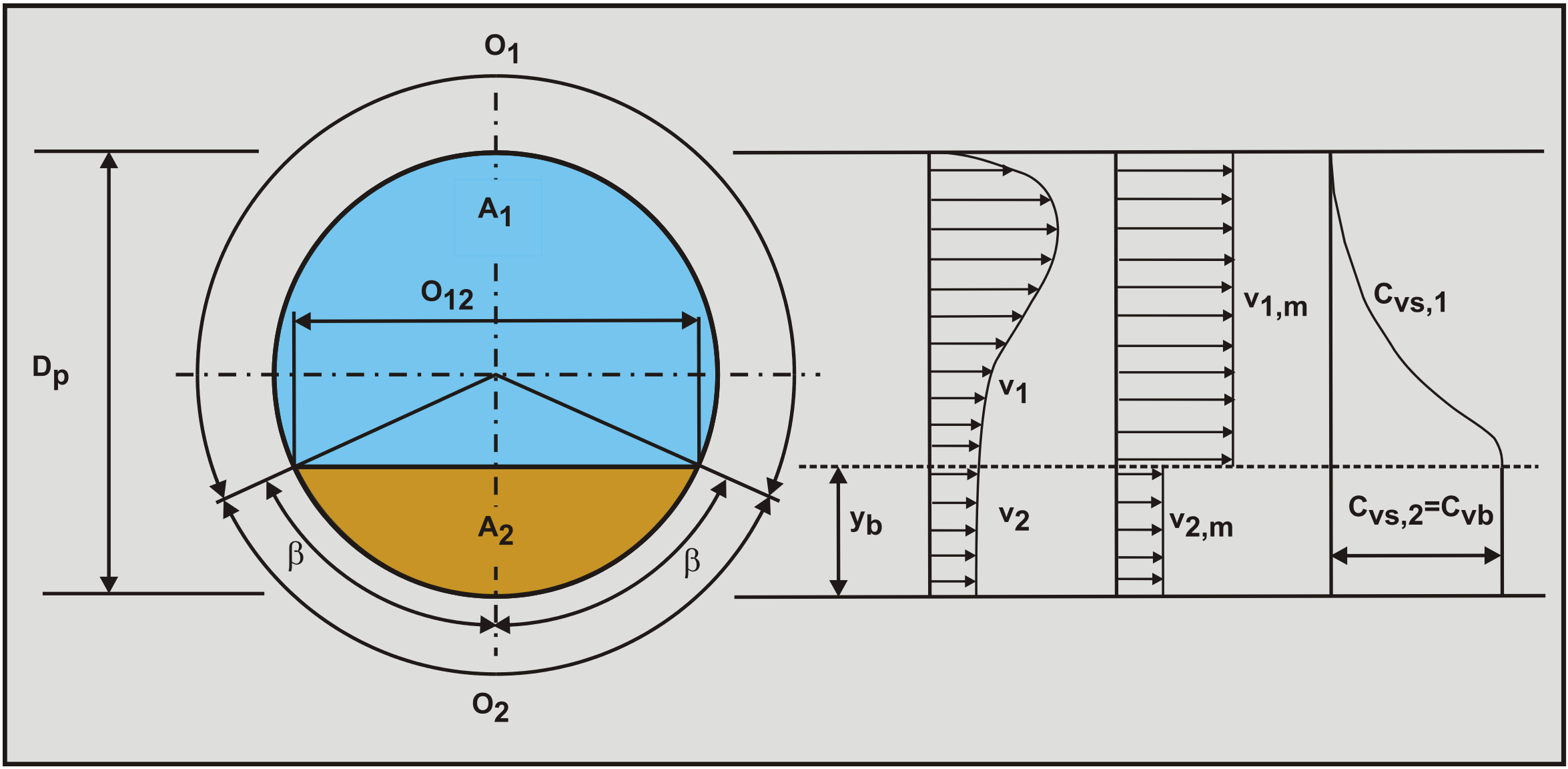
7.4.1 The Friction Force on the Pipe Wall

The friction force F_sf between the bed and the pipe wall equals the normal force F_n on the pipe wall times the friction coefficient μ_sf, giving:

\[\ \mathrm{F}_{\mathrm{s f}}=\mu_{\mathrm{s f}} \cdot \mathrm{F}_{\mathrm{n}}\]

The normal force F_n on the pipe wall is the normal stress σ_n on the pipe wall, integrated over the contact angle β of the bed with the pipe wall.

\[\ \mathrm{F}_{\mathrm{n}}=\Delta \mathrm{L} \cdot \int_{-\beta}^{\beta} \sigma_{\mathrm{n}} \cdot \mathrm{R} \cdot \mathrm{d} \alpha=\Delta \mathrm{L} \cdot \frac{\mathrm{D}_{\mathrm{p}}}{2} \cdot \int_{-\boldsymbol{\beta}}^{\beta} \sigma_{\mathrm{n}} \cdot \mathrm{d} \alpha=\Delta \mathrm{L} \cdot \mathrm{D}_{\mathrm{p}} \cdot \int_{\mathrm{0}}^{\beta} \sigma_{\mathrm{n}} \cdot \mathrm{d} \alpha\]

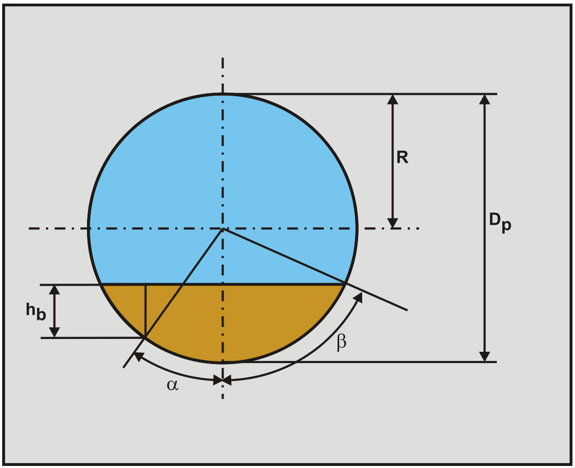
The vertical stress σ_v at an angle α with the vertical can be derived from the height of the bed h_b at that location for β≤π/2 according to Figure 7.4-2:

\[\ \mathrm{h}_{\mathrm{b}}=\mathrm{R} \cdot(\cos (\alpha)-\cos (\beta))=\frac{\mathrm{D}_{\mathrm{p}}}{2} \cdot(\cos (\alpha)-\cos (\beta))\]

The vertical stress σ_v is the submerged weight per unit of area at the specific location at the pipe wall.

\[\ \sigma_{\mathrm{v}}=\rho_{\mathrm{l}} \cdot \mathrm{g} \cdot \mathrm{R}_{\mathrm{sd}} \cdot \mathrm{C}_{\mathrm{vb}} \cdot \frac{\mathrm{D}_{\mathrm{p}}}{2} \cdot(\cos (\alpha)-\cos (\beta))\]

It should be mentioned that the height h_b is different for an angle β≤π/2. For β≤π/2 there are two cases.

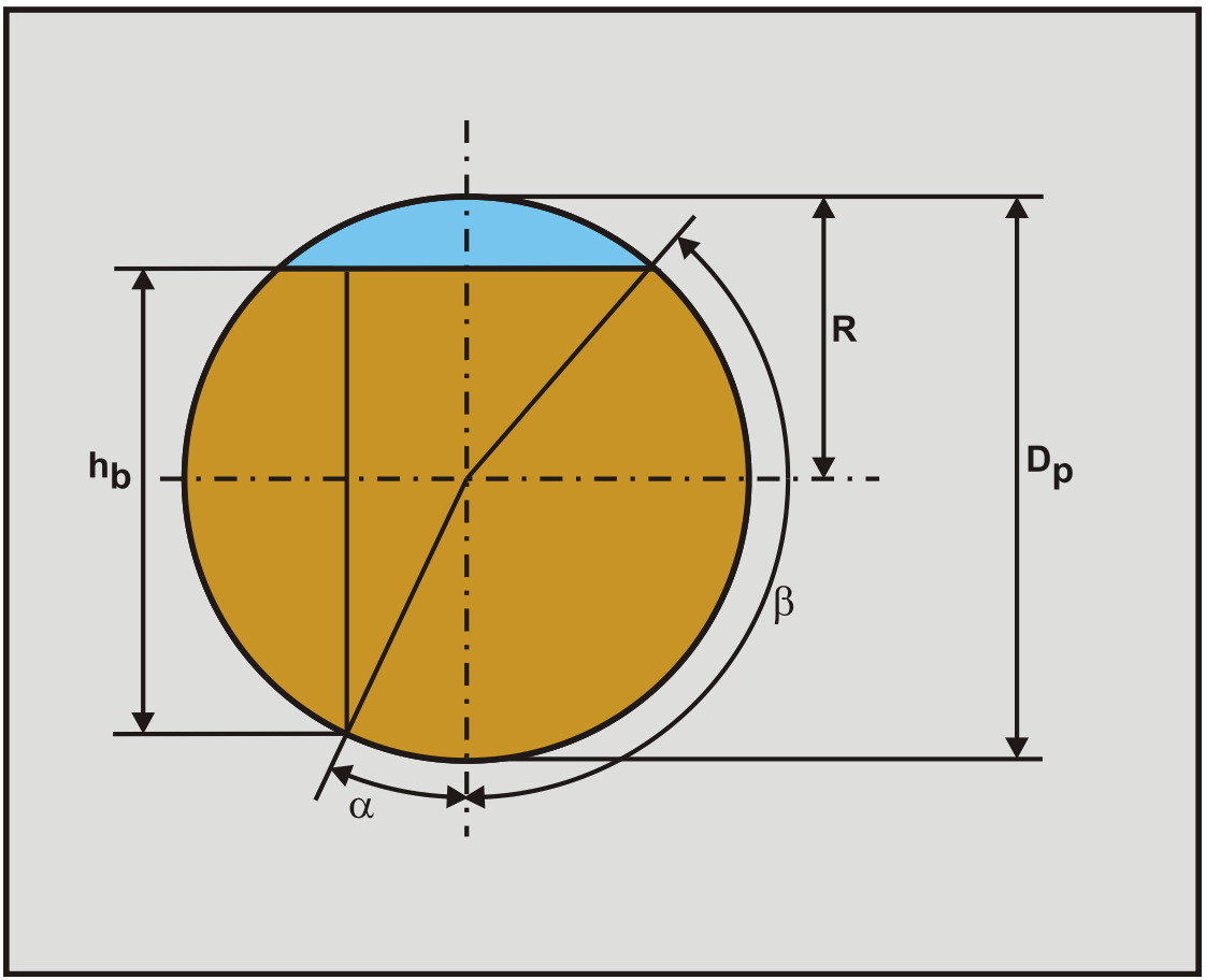
For 0≤α<π-β the vertical stress is based on the distance from the pipe wall at angle α to the free surface of the bed according to Figure 7.4-7, giving for the height of the bed column:

\[\ \mathrm{h_{b}}=\mathrm{R} \cdot(\cos (\alpha)-\cos (\beta))=\frac{\mathrm{D_{p}}}{2} \cdot(\cos (\alpha)-\cos (\beta))\]

And for the vertical normal stress:

\[\ \sigma_{\mathrm{v}}=\rho_{\mathrm{l}} \cdot \mathrm{g} \cdot \mathrm{R}_{\mathrm{sd}} \cdot \mathrm{C}_{\mathrm{vb}} \cdot(\cos (\alpha)-\cos (\beta)) \cdot \frac{\mathrm{D}_{\mathrm{p}}}{2}\]

Figure 7.4-2: The location of an element at the pipe wall and the height of the bed column.

Figure 7.4-3: An element at the pipe wall.

Figure 7.4-4: The stresses at and near the pipe wall.

Figure 7.4-5: The forces at and near the pipe wall.

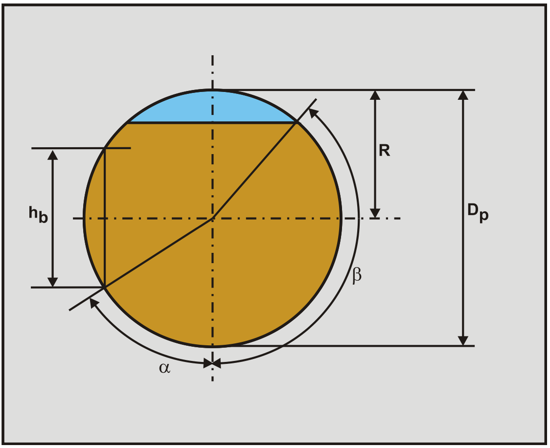
For π-β<α<π/2 the normal stress is based on the two times distance from the pipe wall at angle α to the center line of the pipe according to Figure 7.4-6, giving for the height of the bed column:

\[\ \mathrm{h}_{\mathrm{b}}=\mathrm{2} \cdot \mathrm{R} \cdot \cos (\alpha)=\mathrm{D}_{\mathrm{p}} \cdot \cos (\alpha)\]

And for the vertical normal stress:

\[\ \sigma_{\mathrm{v}}=\rho_{\mathrm{l}} \cdot \mathrm{g} \cdot \mathrm{R_{s d}} \cdot \mathrm{C_{v b}} \cdot 2 \cdot \cos (\alpha) \cdot \frac{\mathrm{D_{p}}}{2}\]

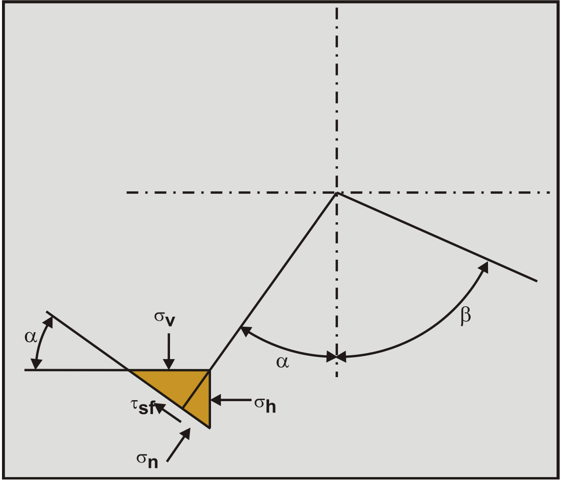
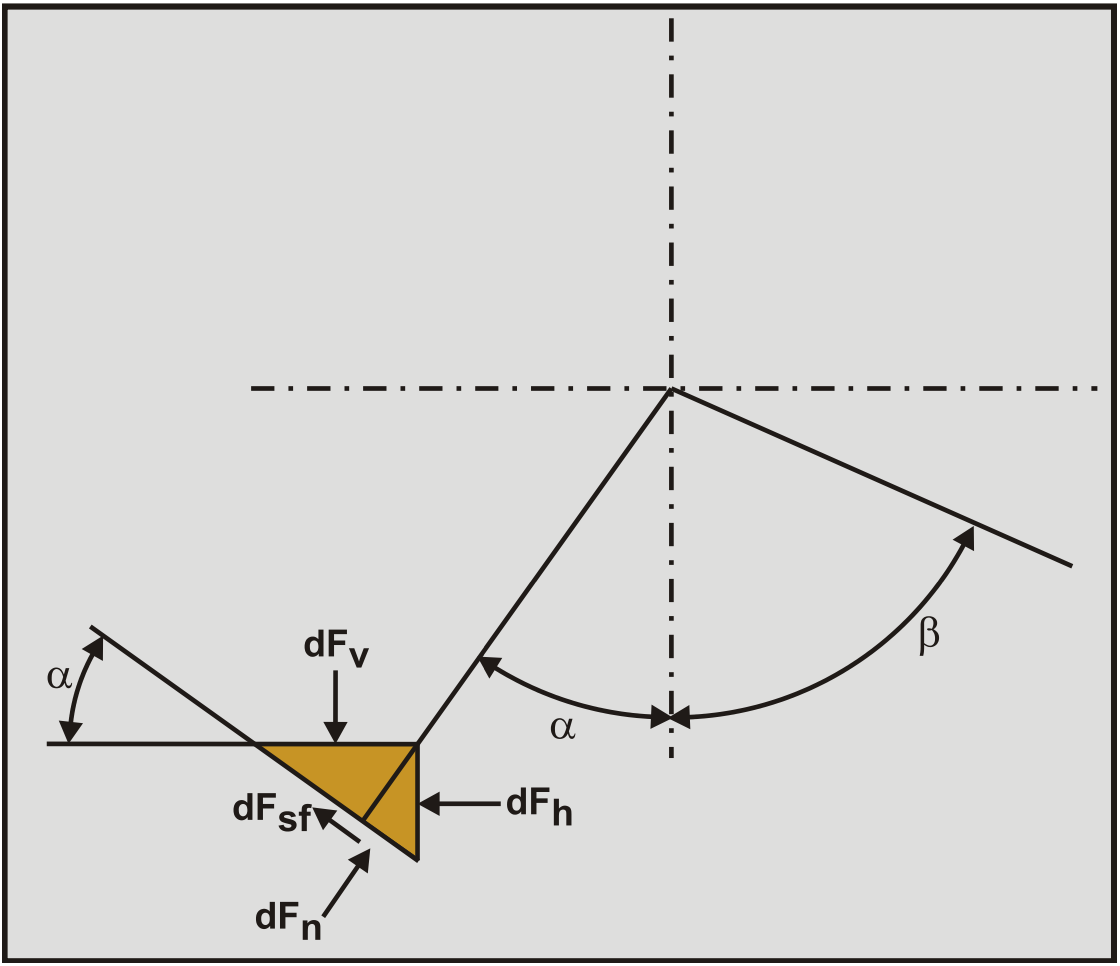
On the bed element at the pipe wall (Figure 7.4-5) there has to be an equilibrium of forces in the horizontal and in the vertical direction, thus for the vertical direction.

\[\ \mathrm{d F}_{\mathrm{n}} \cdot \cos (\alpha)+\mathrm{d F}_{\mathrm{s f}} \cdot \sin (\alpha)=\mathrm{d} \mathrm{F}_{\mathrm{v}}\]

For the horizontal direction this gives:

\[\ \mathrm{d F}_{\mathrm{n}} \cdot \sin (\alpha)-\mathrm{d} \mathrm{F}_{\mathrm{s f}} \cdot \cos (\alpha)=\mathrm{d} \mathrm{F}_{\mathrm{h}}\]

In terms of stresses this gives for the vertical equilibrium:

\[\ \mathrm{\sigma_{n} \cdot \cos (\alpha) \cdot R \cdot d \alpha+\tau_{s f} \cdot \sin (\alpha) \cdot R \cdot d \alpha=\sigma_{v} \cdot R \cdot d \alpha \cdot \cos (\alpha)}\]

For the horizontal equilibrium this gives:

\[\ \mathrm{\sigma_{n} \cdot \sin (\alpha) \cdot \mathrm{R} \cdot \mathrm{d} \alpha-\tau_{s f} \cdot \cos (\alpha) \cdot \mathrm{R} \cdot \mathrm{d} \alpha=\sigma_{h} \cdot \mathrm{R} \cdot \mathrm{d} \alpha \cdot \sin (\alpha)}\]

With the relation between the normal stress and the shear stress:

\[\ \tau_{\mathrm{s f}}=\mu_{\mathrm{s f}, \mathrm{e}} \cdot \sigma_{\mathrm{n}}\]

This gives for the vertical equilibrium:

\[\ \mathrm{\sigma_{n} \cdot\left(\cos (\alpha)+\mu_{s f, e} \cdot \sin (\alpha)\right) \cdot R \cdot d \alpha}=\mathrm{\sigma_{v} \cdot R \cdot d \alpha \cdot \cos (\alpha)}\]

For the horizontal equilibrium this gives:

\[\ \mathrm{\sigma_{n} \cdot\left(\sin (\alpha)-\mu_{\mathrm{sf}, \mathrm{e}} \cdot \cos (\alpha)\right) \cdot \mathrm{R} \cdot \mathrm{d} \alpha}=\sigma_{\mathrm{h}} \cdot \mathrm{R} \cdot \mathrm{d} \alpha \cdot \sin (\alpha)\]

Since friction is always in the opposite direction of the interface velocity, 3 cases can be distinguished:

1. The bed is stationary and the liquid above the bed is also stationary. Since there is no velocity in any direction, the friction can be mobilized between 0 and a maximum value in any direction, counteracting forces that may occur. Since in this case the only force is the gravitational force, there may be friction between the bed and the pipe wall counteracting gravity with a maximum of μ_sf,e= μ_sf.
2. The bed is stationary, but the liquid above the bed has a certain velocity resulting in a shear stress and thus shear force on the bed. There will be a friction force between the bed and the pipe wall counteracting the shear force on the bed, but this does not mean the friction is fully mobilized. There may still be some friction capacity left counteracting gravity in the cross section of the pipe.
3. The bed is sliding. The friction force on the bed is opposite to the velocity of the bed. There is no friction mobilized in the cross section of the pipe, so μ_sf,e=0.

When the line speed increases from 0 m/sec to a line speed above the Limit of Stationary Deposit Velocity, the friction undergoes a transition from mobilization in the cross section of the pipe counteracting gravity, to mobilization in the longitudinal direction of the pipe counteracting shear and pressure. Since the effective mobilized friction is only known in the case of a sliding bed, first a generic solution will be derived for the normal force between the bed and the pipe wall, taking into consideration that the integrated vertical components of the normal force and the wall friction force should always be equal to the weight of the bed.

7.4.2 The Active/Passive Soil Failure Approach

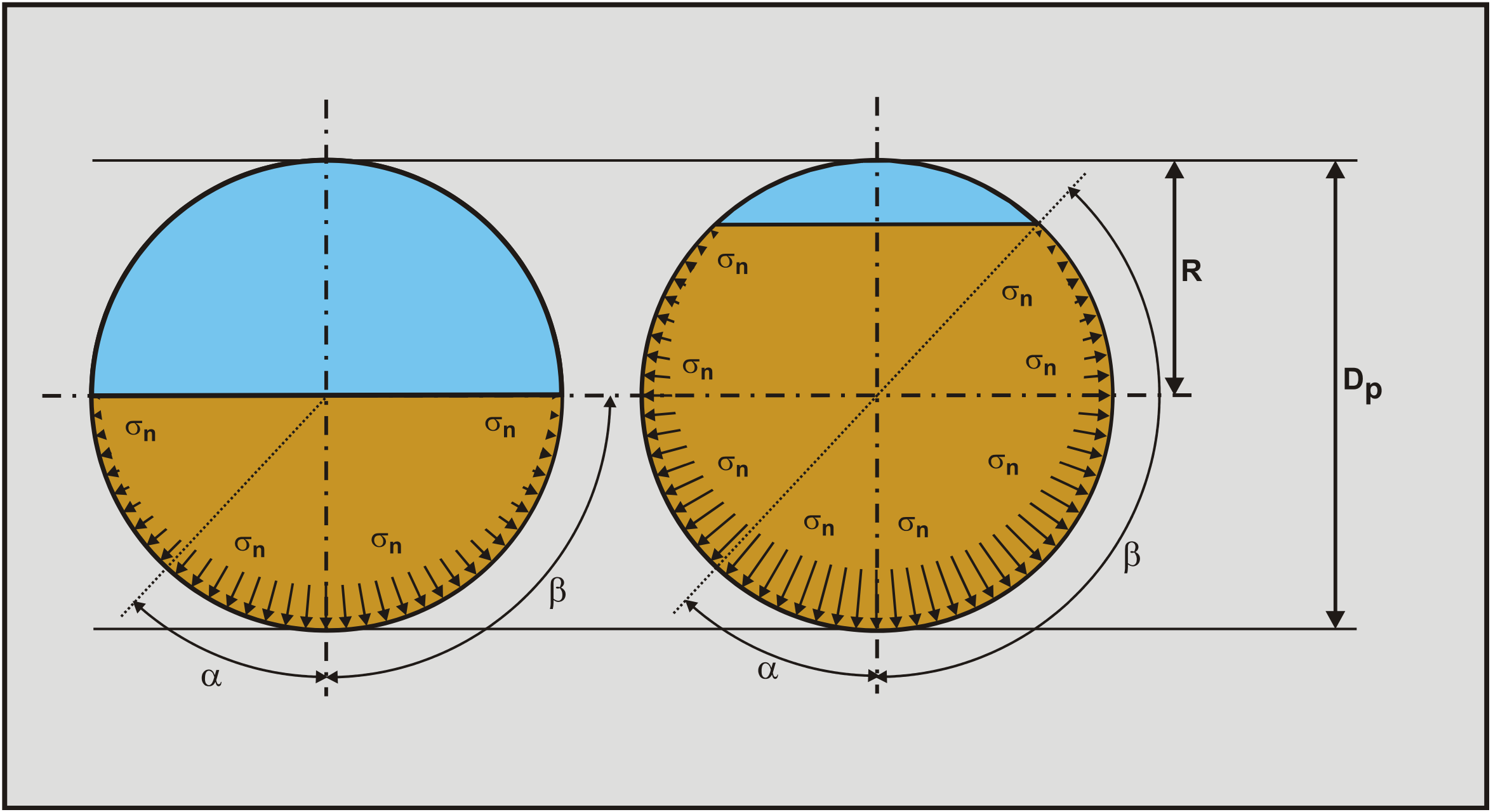
Given a vertical stress σ_v at the pipe wall according to equation (7.4-4) for the case where β≤π/2 and equations (7.4-6) and (7.4-8) for the case where β>π/2 and considering that the vertical stress σ_v is only present in the bottom half of the pipe, it can be assumed that the horizontal stress σ_h is a factor K times the vertical stress σ_v. According to soil mechanics, this factor K should be in between the factor for active failure K_a and the factor for passive failure K_p. These two factors depend on the angle of internal friction of the sand bed φ, which for a loose packed bed will have a value near 30o. The K_a value is 1/3 and the K_p value 3 for an internal friction angle of 30o. The K value cannot be smaller than K_a or bigger than K_p.

The coefficients for active K_a and passive K_p failure are:

\[\ \mathrm{K_{a}=\frac{1-\sin (\varphi)}{1+\sin (\varphi)} \quad\text{ and }\quad K_{p}=\frac{1+\sin (\varphi)}{1-\sin (\varphi)}}\]

This gives for the horizontal stress σ_h near the pipe wall:

\[\ \sigma_{\mathrm{h}}=\mathrm{K} \cdot \sigma_{\mathrm{v}}\]

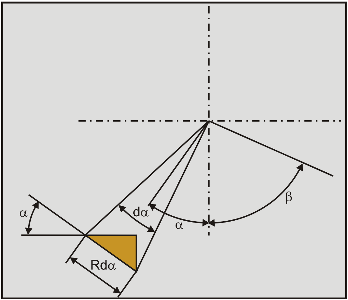
The forces on an element R·dα on the pipe wall per unit of pipe length are now:

\[\ \mathrm{d F}_{\mathrm{v}}=\sigma_{\mathrm{v}} \cdot \cos (\alpha) \cdot \mathrm{R} \cdot \mathrm{d} \mathrm{\alpha} \cdot \Delta \mathrm{L}\]

\[\ \mathrm{d F}_{\mathrm{h}}=\sigma_{\mathrm{h}} \cdot \sin (\alpha) \cdot \mathrm{R} \cdot \mathrm{d} \mathrm{\alpha} \cdot \Delta \mathrm{L}\]

The components of these forces normal to the pipe wall are:

\[\ \mathrm{d F}_{\mathrm{v}, \mathrm{n}}=\sigma_{\mathrm{v}} \cdot \cos (\alpha) \cdot \mathrm{R} \cdot \mathrm{d} \alpha \cdot \cos (\alpha) \cdot \Delta \mathrm{L}\]

\[\ \mathrm{d F}_{\mathrm{h}, \mathrm{n}}=\sigma_{\mathrm{h}} \cdot \sin (\alpha) \cdot \mathrm{R} \cdot \mathrm{d} \alpha \cdot \sin (\alpha) \cdot \Delta \mathrm{L}\]

This gives for the normal force on an element R·dα on the pipe wall:

\[\ \mathrm{d F}_{\mathrm{n}}=\mathrm{d F}_{\mathrm{v}, \mathrm{n}}+\mathrm{d} \mathrm{F}_{\mathrm{h}, \mathrm{n}}=\sigma_{\mathrm{v}} \cdot \cos ^{2}(\alpha) \cdot \mathrm{R} \cdot \mathrm{d} \alpha \cdot \Delta \mathrm{L}+\sigma_{\mathrm{h}} \cdot \sin ^{2}(\alpha) \cdot \mathrm{R} \cdot \mathrm{d} \alpha \cdot \Delta \mathrm{L}\]

Substituting equation (7.4-17) gives:

\[\ \mathrm{d F}_{\mathrm{n}}=\mathrm{d F}_{\mathrm{v}, \mathrm{n}}+\mathrm{d} \mathrm{F}_{\mathrm{h}, \mathrm{n}}=\sigma_{\mathrm{v}} \cdot\left(\cos ^{2}(\alpha)+\mathrm{K} \cdot \sin ^{2}(\alpha)\right) \cdot \mathrm{R} \cdot \mathrm{d} \alpha \cdot \Delta \mathrm{L}\]

The normal stress on the pipe wall is now:

\[\ \sigma_{\mathrm{n}}=\frac{\mathrm{dF}_{\mathrm{n}}}{\mathrm{R} \cdot \mathrm{d} \alpha \cdot \Delta \mathrm{L}}=\frac{\mathrm{dF}_{\mathrm{v}, \mathrm{n}}+\mathrm{d} \mathrm{F}_{\mathrm{h}, \mathrm{n}}}{\mathrm{R} \cdot \mathrm{d} \alpha \cdot \Delta \mathrm{L}}=\sigma_{\mathrm{v}} \cdot\left(\cos ^{2}(\alpha)+\mathrm{K} \cdot \sin ^{2}(\alpha)\right)\]

To determine the total normal force F_n on the pipe wall, this normal stress has to be integrated. Two cases have to be considered. The first case considers a bed which occupies less than or equal to 50% of the pipe, so β≤π/2. The second case considers a bed which occupies more than 50% of the pipe, so β>π/2.

Case 1: β≤π/2

For 0≤α<β the normal stress is based on the distance from the pipe wall at angle α to the free surface of the bed as is shown in Figure 7.4-2, giving:

\[\ \sigma_{\mathrm{n}}=\rho_{\mathrm{l}} \cdot \mathrm{R}_{\mathrm{s d}} \cdot \mathrm{g} \cdot \mathrm{C}_{\mathrm{v b}} \cdot \mathrm{R} \cdot(\cos (\alpha)-\cos (\beta)) \cdot\left(\mathrm{K} \cdot \sin ^{2}(\alpha)+\cos ^{2}(\alpha)\right)\]

Integrating from α=0 to α=β and multiplying by 2 for the left and right side gives for the normal force:

\[\ \mathrm{F}_{\mathrm{n}}=\mathrm{2} \cdot \rho_{\mathrm{l}} \cdot \mathrm{R}_{\mathrm{s d}} \cdot \mathrm{g} \cdot \mathrm{C}_{\mathrm{v b}} \cdot \mathrm{R}^{2} \cdot \int_{\mathrm{0}}^{\beta}(\cos (\alpha)-\cos (\beta)) \cdot\left(\mathrm{K} \cdot \sin ^{2}(\alpha)+\cos ^{2}(\alpha)\right) \cdot \mathrm{d} \alpha \cdot \Delta \mathrm{L}\]

Substituting the upper and lower boundary gives:

\[\ \mathrm{F}_{\mathrm{n}}=\mathrm{2} \cdot \rho_{\mathrm{l}} \cdot \mathrm{R}_{\mathrm{s d}} \cdot \mathrm{g} \cdot \mathrm{C}_{\mathrm{v b}} \cdot \mathrm{R}^{2} \cdot\left(\frac{\mathrm{K}-\mathrm{1}}{\mathrm{3}} \cdot \sin ^{3}(\beta)+\sin (\beta)-\frac{\mathrm{K}+\mathrm{1}}{2} \cdot \beta \cdot \cos (\beta)+\frac{\mathrm{K}-\mathrm{1}}{2} \cdot \sin (\beta) \cdot \cos ^{2}(\beta)\right) \cdot \Delta \mathrm{L}\]

Case 2: β>π/2

Figure 7.4-6: The height of the bed column for π-β<α<π/2.

Figure 7.4-7: The height of the bed column for 0≤α<π-β.

For 0≤α<π-β the normal stress is based on the distance from the pipe wall at angle α to the free surface of the bed, giving:

\[\ \sigma_{\mathrm{n}}=\rho_{\mathrm{l}} \cdot \mathrm{R}_{\mathrm{s d}} \cdot \mathrm{g} \cdot \mathrm{C}_{\mathrm{v b}} \cdot \mathrm{R} \cdot(\cos (\alpha)-\cos (\beta)) \cdot\left(\mathrm{K} \cdot \sin ^{2}(\alpha)+\cos ^{2}(\alpha)\right)\]

For π-β<α<π/2 the normal stress is based on the two times distance from the pipe wall at angle α to the center line of the pipe, giving:

\[\ \sigma_{\mathrm{n}}=\rho_{\mathrm{l}} \cdot \mathrm{R}_{\mathrm{sd}} \cdot \mathrm{g} \cdot \mathrm{C}_{\mathrm{v b}} \cdot \mathrm{R} \cdot \mathrm{2} \cdot \cos (\alpha) \cdot\left(\mathrm{K} \cdot \sin ^{2}(\alpha)+\cos ^{2}(\alpha)\right)\]

Integrating from α=0 to α= π/2 gives for the normal force:

\[\ \begin{array}{left}\mathrm{F_{n}}&=\mathrm{2 \cdot \rho_{l} \cdot R_{s d} \cdot g \cdot C_{v b} \cdot R^{2} \cdot \int_{0}^{\pi-\beta}(\cos (\alpha)-\cos (\beta)) \cdot\left(K \cdot \sin ^{2}(\alpha)+\cos ^{2}(\alpha)\right) \cdot d \alpha \cdot \Delta L}\\
&\mathrm{+2 \cdot \rho_{l} \cdot R_{s d} \cdot g \cdot C_{v b} \cdot R^{2} \cdot \int_{\pi-\beta}^{\pi / 2} 2 \cdot \cos (\alpha) \cdot\left(K \cdot \sin ^{2}(\alpha)+\cos ^{2}(\alpha)\right) \cdot d \alpha \cdot \Delta L}\end{array}\]

Substituting the upper and lower boundaries gives:

\[\ \mathrm{F_n = 2 \cdot \rho_l \cdot R_{sd} \cdot g \cdot C_{vb} \cdot R^2 \cdot}\Delta \mathrm{L} \cdot\left(\begin{array}{l}\frac{\mathrm{K}-\mathrm{1}}{\mathrm{3}} \cdot \sin ^{3}(\beta)+\sin (\beta)-\frac{\mathrm{K}+\mathrm{1}}{2} \cdot(\pi-\beta) \cdot \cos (\beta)-\frac{\mathrm{K}-\mathrm{1}}{2} \cdot \sin (\beta) \cdot \cos ^{2}(\beta) \\ +\frac{2}{3} \cdot(\mathrm{K}-1)+2-\frac{2}{3} \cdot(\mathrm{K}-1) \cdot \sin ^{3}(\beta)-2 \cdot \sin (\beta)\end{array}\right)\]

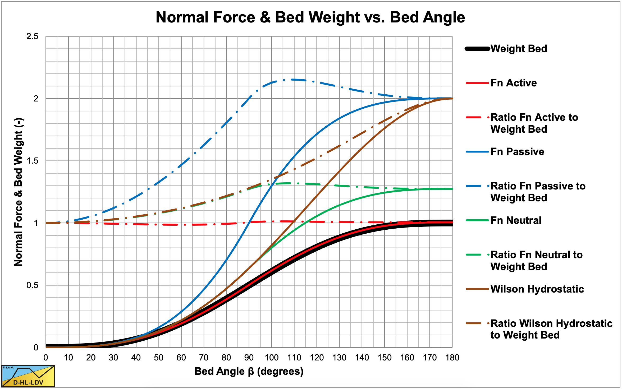
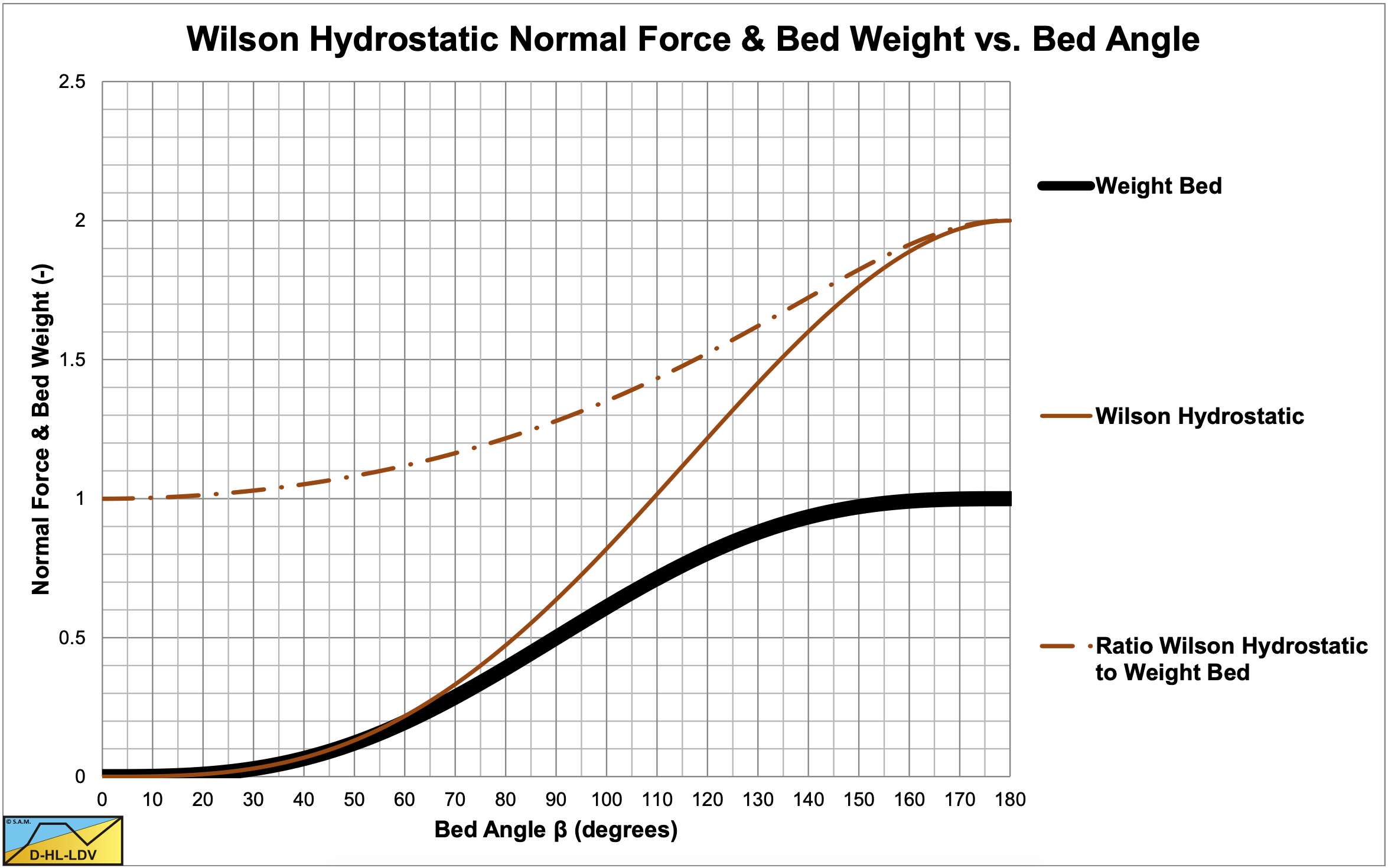
Figure 7.4-8 Shows the results of equations (7.4-27) and (7.4-31) for the cases of active failure K=K_a, passive failure K=K_p and neutral K=1 for an angle of internal friction of φ=27.5^o. The figure also shows the weight of the bed and the ratio between the normal force and the weight for all cases.

Figure 7.4-8: The normal force in relation to the bed fraction and the bed angle (φ=27.5^o).

The components of these forces tangent to the pipe wall are:

\[\ \mathrm{d} \mathrm{F}_{\mathrm{v}, \mathrm{t}}=\sigma_{\mathrm{v}} \cdot \cos (\alpha) \cdot \mathrm{R} \cdot \mathrm{d} \alpha \cdot \sin (\alpha) \cdot \Delta \mathrm{L}\]

\[\ \mathrm{d F}_{\mathrm{h}, \mathrm{t}}=-\sigma_{\mathrm{h}} \cdot \sin (\alpha) \cdot \mathrm{R} \cdot \mathrm{d} \alpha \cdot \cos (\alpha) \cdot \Delta \mathrm{L}\]

This gives for the tangent force on an element R·dα on the pipe wall:

\[\ \mathrm{d F}_{\mathrm{t}}=\mathrm{d F}_{\mathrm{v}, \mathrm{t}}+\mathrm{d F}_{\mathrm{h}, \mathrm{t}}=\sigma_{\mathrm{v}} \cdot \sin (\alpha) \cdot \cos (\alpha) \cdot \mathrm{R} \cdot \mathrm{d} \mathrm{\alpha} \cdot \Delta \mathrm{L}-\sigma_{\mathrm{h}} \cdot \sin (\alpha) \cdot \cos (\alpha) \cdot \mathrm{R} \cdot \mathrm{d} \alpha \cdot \Delta \mathrm{L}\]

Substituting equation (7.4-17) gives:

\[\ \mathrm{d} \mathrm{F}_{\mathrm{t}}=\mathrm{d} \mathrm{F}_{\mathrm{v}, \mathrm{t}}+\mathrm{d} \mathrm{F}_{\mathrm{h}, \mathrm{t}}=\sigma_{\mathrm{v}} \cdot \sin (\alpha) \cdot \cos (\alpha) \cdot(\mathrm{1}-\mathrm{K}) \cdot \mathrm{R} \cdot \mathrm{d} \alpha \cdot \Delta \mathrm{L}\]

The tangential or friction stress on the pipe wall is now:

\[\ \tau_{\mathrm{sf}}=\tau_{\mathrm{t}}=\frac{\mathrm{d} \mathrm{F}_{\mathrm{t}}}{\mathrm{R} \cdot \mathrm{d} \alpha \cdot \Delta \mathrm{L}}=\frac{\mathrm{d} \mathrm{F}_{\mathrm{v}, \mathrm{t}}+\mathrm{d} \mathrm{F}_{\mathrm{h}, \mathrm{t}}}{\mathrm{R} \cdot \mathrm{d} \alpha \cdot \Delta \mathrm{L}}=\sigma_{\mathrm{v}} \cdot \sin (\alpha) \cdot \cos (\alpha) \cdot(1-\mathrm{K})=\mu_{\mathrm{sf}, \mathrm{e}} \cdot \sigma_{\mathrm{n}}\]

With:

\[\ \sigma_{\mathrm{n}}=\frac{\mathrm{dF}_{\mathrm{n}}}{\mathrm{R} \cdot \mathrm{d} \alpha \cdot \Delta \mathrm{L}}=\frac{\mathrm{d} \mathrm{F}_{\mathrm{v}, \mathrm{n}}+\mathrm{d} \mathrm{F}_{\mathrm{h}, \mathrm{n}}}{\mathrm{R} \cdot \mathrm{d} \alpha \cdot \Delta \mathrm{L}}=\sigma_{\mathrm{v}} \cdot\left(\cos ^{2}(\alpha)+\mathrm{K} \cdot \sin ^{2}(\alpha)\right)\]

Giving:

\[\ \sin (\alpha) \cdot \cos (\alpha) \cdot(1-\mathrm{K})=\mu_{\mathrm{sf}, \mathrm{e}} \cdot\left(\cos ^{2}(\alpha)+\mathrm{K} \cdot \sin ^{2}(\alpha)\right)\]

The K factor is related to the wall friction coefficient according to:

\[\ \mathrm{K}=\frac{\sin (\alpha) \cdot \cos (\alpha)-\mu_{\mathrm{sf}, \mathrm{e}} \cdot \cos ^{2}(\alpha)}{\sin (\alpha) \cdot \cos (\alpha)+\mu_{\mathrm{sf}, \mathrm{e}} \cdot \sin ^{2}(\alpha)}\]

In the case of a sliding bed, there is no friction in the cross section of the pipe (Figure 7.4-4), so the only solution is K=1, which is the neutral curve for the normal force F_n as a function of the angle β in Figure 7.4-8. In the case of a stationary bed, the relation between the factor K and the effective sliding friction coefficient μ_sf,e depends on the angle α, no general solution exists. K=1 will simplify the equations and also appears to be to correct value for K to ensure that the vertical component of the normal stress will carry the submerged weight of the bed. The resulting normal force Fn is bigger than the weight of the bed, starting with a factor 1 for a β=0, increasing to a factor of 1.27 at β=π/2, increasing to a maximum of 1.32 at β=0.6·π and after that decreasing slowly to 1.27 at β=π. So above β=π/2 the factor is almost constant with an average value of 1.293.

7.4.3 The Hydrostatic Normal Stress Distribution Approach

Figure 7.4-9: The hydrostatic normal stress distribution according to Wilson et al. (1992).

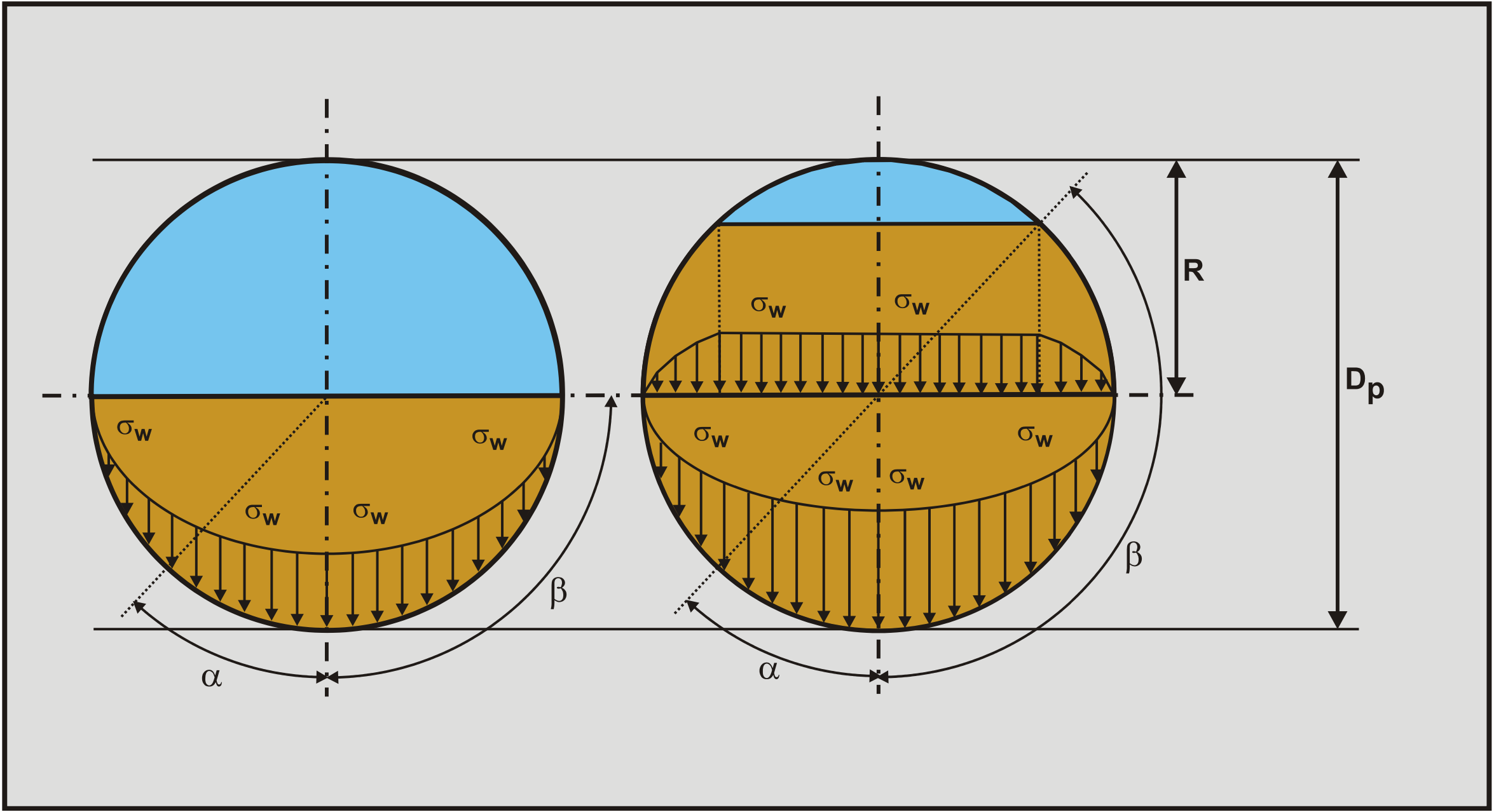
Wilson et al. (1992) assume a hydrostatic normal stress distribution on the pipe wall as if the bed was a liquid as is shown in Figure 7.4-9. The left picture shows the normal stress distribution up to a bed angle β of π/2, the right picture for β > π/2. The normal stress as a function of the angle α, given a bed angle β can be expressed by:

\[\ \sigma_{\mathrm{n}}=\rho_{\mathrm{l}} \cdot \mathrm{g} \cdot \mathrm{R}_{\mathrm{sd}} \cdot \mathrm{C}_{\mathrm{vb}} \cdot \frac{\mathrm{D}_{\mathrm{p}}}{2} \cdot(\cos (\alpha)-\cos (\beta))\]

This is different from the assumption that the friction force F_sf equals the submerged weight F_W times the sliding friction coefficient μ_sf.

The total normal force F_N follows from integration of the normal stress:

\[\ \begin{array}{left} \mathrm{F}_{\mathrm{n}}&=\Delta \mathrm{L} \cdot \int_{-\beta}^{\beta} \sigma_{\mathrm{n}} \cdot \mathrm{R} \cdot \mathrm{d} \alpha=2 \cdot \Delta \mathrm{L} \cdot \int_{\mathrm{0}}^{\beta} \rho_{\mathrm{l}} \cdot \mathrm{g} \cdot \mathrm{R}_{\mathrm{s} \mathrm{d}} \cdot \mathrm{C}_{\mathrm{v} \mathrm{b}} \cdot \frac{\mathrm{D}_{\mathrm{p}}^{2}}{4} \cdot(\cos (\alpha)-\cos (\beta)) \cdot \mathrm{d} \alpha\\
&=\rho_{\mathrm{l}} \cdot \mathrm{g} \cdot \Delta \mathrm{L} \cdot \mathrm{R}_{\mathrm{s} \mathrm{d}} \cdot \mathrm{C}_{\mathrm{v} \mathrm{b}} \cdot \frac{\mathrm{D}_{\mathrm{p}}^{2}}{2} \cdot \int_{0}^{\beta}(\cos (\alpha)-\cos (\beta)) \cdot \mathrm{d} \alpha\end{array}\]

This gives for the normal force F_N:

\[\ \mathrm{F}_{\mathrm{n}}=\rho_{\mathrm{l}} \cdot \mathrm{g} \cdot \mathrm{\Delta} \mathrm{L} \cdot \mathrm{R}_{\mathrm{s d}} \cdot \mathrm{C}_{\mathrm{v b}} \cdot \frac{\mathrm{D}_{\mathrm{p}}^{2}}{\mathrm{2}} \cdot(\sin (\beta)-\boldsymbol{\beta} \cdot \cos (\boldsymbol{\beta}))\]

So the sliding friction force is:

\[\ \mathrm{F}_{\mathrm{s f}}=\mathrm{2} \cdot \mu_{\mathrm{s f}} \cdot \rho_{\mathrm{l}} \cdot \mathrm{g} \cdot \Delta \mathrm{L} \cdot \mathrm{R}_{\mathrm{s d}} \cdot \mathrm{C}_{\mathrm{v b}} \cdot \mathrm{A}_{\mathrm{p}} \cdot \frac{(\sin (\beta)-\beta \cdot \cos (\beta))}{\pi}\]

The submerged weight of the bed F_w is given by:

\[\ \mathrm{F}_{\mathrm{w}}=\rho_{\mathrm{l}} \cdot \mathrm{g} \cdot \Delta \mathrm{L} \cdot \mathrm{R}_{\mathrm{s d}} \cdot \mathrm{C}_{\mathrm{v b}} \cdot \mathrm{A}_{\mathrm{p}} \cdot \frac{(\beta-\sin (\beta) \cdot \cos (\beta))}{\pi}\]

So the ratio between the normal force and the submerged weight is:

\[\ \mathrm{\frac{F_{n}}{F_{w}}=\frac{2 \cdot(\sin (\beta)-\beta \cdot \cos (\beta))}{(\beta-\sin (\beta) \cdot \cos (\beta))}}\]

For small values of β, up to 60 degrees, this ratio is just above 1. But at larger angles (larger concentrations), this ratio is bigger than 1, with a maximum of 2 when the whole pipe is occupied with a bed and β=π.

Figure 7.4-10: The normal force F_n, the submerged weight F_w and the ratio F_n/F_w.

The pressure losses due to the sliding friction of the bed based on the hydrostatic normal stress distribution are now:

\[\ \Delta \mathrm{p}_{\mathrm{m}}-\Delta \mathrm{p}_{\mathrm{l}}=\frac{\mathrm{F}_{\mathrm{s f}}}{\mathrm{A}_{\mathrm{p}}}=\frac{\mu_{\mathrm{s f}} \cdot \mathrm{F}_{\mathrm{n}}}{\frac{\pi}{\mathrm{4}} \cdot \mathrm{D}_{\mathrm{p}}^{2}}=\mathrm{2} \cdot \mu_{\mathrm{s f}} \cdot \rho_{\mathrm{l}} \cdot \mathrm{g} \cdot \Delta \mathrm{L} \cdot \mathrm{R}_{\mathrm{s d}} \cdot \mathrm{C}_{\mathrm{v b}} \cdot \frac{(\sin (\beta)-\beta \cdot \cos (\beta))}{\pi}\]

This gives for the hydraulic gradient:

\[\ \mathrm{i}_{\mathrm{m}}-\mathrm{i}_{\mathrm{l}}=\frac{\mathrm{F}_{\mathrm{s f}}}{\mathrm{A}_{\mathrm{p}} \cdot \rho_{\mathrm{l}} \cdot \mathrm{g} \cdot \Delta \mathrm{L}}=\frac{\mu_{\mathrm{s f}} \cdot \mathrm{F}_{\mathrm{n}}}{\frac{\pi}{4} \cdot \mathrm{D}_{\mathrm{p}}^{2} \cdot \rho_{\mathrm{l}} \cdot \mathrm{g} \cdot \Delta \mathrm{L}}=\mathrm{2} \cdot \mu_{\mathrm{s f}} \cdot \mathrm{R}_{\mathrm{s d}} \cdot \mathrm{C}_{\mathrm{v b}} \cdot \frac{(\sin (\beta)-\beta \cdot \cos (\beta))}{\pi}\]

In the case where the bed occupies the whole pipe cross section, β=π, this gives the so called plug gradient:

\[\ \mathrm{i}_{\mathrm{p} \operatorname{lug}}=\mathrm{i}_{\mathrm{m}}-\mathrm{i}_{\mathrm{l}}=\mathrm{2} \cdot \mu_{\mathrm{s f}} \cdot \mathrm{R}_{\mathrm{s d}} \cdot \mathrm{C}_{\mathrm{v b}} \cdot \frac{(\sin (\pi)-\pi \cdot \cos (\pi))}{\pi}=\mathrm{2} \cdot \mu_{\mathrm{s f}} \cdot \mathrm{R}_{\mathrm{s d}} \cdot \mathrm{C}_{\mathrm{v b}}\]

This gives for the relative excess hydraulic gradient E_rhg:

\[\ \mathrm{E}_{\mathrm{rhg}}=\frac{\mathrm{i}_{\mathrm{m}}-\mathrm{i}_{\mathrm{l}}}{\mathrm{R}_{\mathrm{sd}} \cdot \mathrm{C}_{\mathrm{v} \mathrm{s}}}=\mu_{\mathrm{sf}} \cdot \frac{2 \cdot(\sin (\beta)-\beta \cdot \cos (\beta))}{(\beta-\sin (\beta) \cdot \cos (\beta))}\]

7.4.4 The Normal Force Carrying the Weight Approach

With this approach it is assumed that there can only be a normal force between the bed and the pipe wall in the bottom half of the pipe. Bed in the top half of the pipe transfers the submerged weight to the bottom half of the pipe. If the bed occupies less than or equal to half of the pipe cross section, the solution is equal to the Wilson et al. (1992) hydrostatic approach. If the bed occupies more than half of the pipe cross section, the solution differs.

Figure 7.4-11: The normal stress and weight distribution.

Figure 7.4-11 shows these two cases. Figure 7.4-2, Figure 7.4-3, Figure 7.4-4 and Figure 7.4-5 show the stresses on the pipe wall.

It is obvious that the vertical component of the normal stress on the pipe wall has to carry the submerged weight of the bed.

The vertical stress as a result of the submerged weight at a point under an angle α is:

\[\ \sigma_{\mathrm{v}}=\rho_{\mathrm{l}} \cdot \mathrm{R}_{\mathrm{sd}} \cdot \mathrm{g} \cdot \mathrm{C}_{\mathrm{vb}} \cdot(\cos (\alpha)-\cos (\beta)) \cdot \mathrm{R}\]

The vertical force exerted on a strip pipe wall with a length ΔL is:

\[\ \Delta \mathrm{F}_{\mathrm{v}}=\sigma_{\mathrm{v}} \cdot \cos (\alpha) \cdot \mathrm{R} \cdot \mathrm{d} \alpha \cdot \Delta \mathrm{L}\]

The normal force exerted on a strip pipe wall with a length ΔL is:

\[\ \Delta \mathrm{F}_{\mathrm{n}}=\sigma_{\mathrm{n}} \cdot \mathrm{R} \cdot \mathrm{d} \mathrm{\alpha} \cdot \mathrm{\Delta} \mathrm{L}\]

The vertical component of the normal force exerted on a strip pipe wall with a length ΔL is:

\[\ \Delta \mathrm{F}_{\mathrm{n}, \mathrm{v}}=\sigma_{\mathrm{n}} \cdot \cos (\alpha) \cdot \mathrm{R} \cdot \mathrm{d} \alpha \cdot \Delta \mathrm{L}\]

The vertical component of the normal force has to be equal to the vertical force resulting from the submerged weight according to:

\[\ \mathrm{\sigma_{n} \cdot \cos (\alpha) \cdot R \cdot d \alpha \cdot \Delta L=\rho_{l} \cdot R_{s d} \cdot g \cdot C_{v b} \cdot(\cos (\alpha)-\cos (\beta)) \cdot R \cdot \cos (\alpha) \cdot R \cdot d \alpha \cdot \Delta L}\]

This can be simplified to:

\[\ \sigma_{\mathrm{n}} \cdot \mathrm{R} \cdot \mathrm{d} \alpha \cdot \Delta \mathrm{L}=\rho_{\mathrm{l}} \cdot \mathrm{R}_{\mathrm{sd}} \cdot \mathrm{g} \cdot \mathrm{C}_{\mathrm{v b}} \cdot(\cos (\alpha)-\cos (\beta)) \cdot \mathrm{R} \cdot \mathrm{R} \cdot \mathrm{d} \alpha \cdot \Delta \mathrm{L}\]

The total normal force follows from integration of the normal stress:

\[\ \mathrm{F}_{\mathrm{n}}=\int_{-\beta}^{\beta} \sigma_{\mathrm{n}} \cdot \mathrm{R} \cdot \mathrm{d} \alpha \cdot \Delta \mathrm{L}=\mathrm{2} \cdot \rho_{\mathrm{l}} \cdot \mathrm{R}_{\mathrm{s} \mathrm{d}} \cdot \mathrm{g} \cdot \mathrm{C}_{\mathrm{v} \mathrm{b}} \cdot \mathrm{R}^{2} \cdot \int_{\mathrm{0}}^{\beta}(\cos (\alpha)-\cos (\beta)) \cdot \mathrm{d} \alpha \cdot \Delta \mathrm{L}\]

Per unit of length and for both sides of the bed this gives:

\[\ \begin{array}{left} \mathrm{F}_{\mathrm{n}}&=\mathrm{2} \cdot \rho_{\mathrm{l}} \cdot \mathrm{R}_{\mathrm{s} \mathrm{d}} \cdot \mathrm{g} \cdot \mathrm{C}_{\mathrm{v} \mathrm{b}} \cdot \mathrm{R}^{2} \cdot(\sin (\beta)-\beta \cdot \cos (\beta)) \cdot \Delta \mathrm{L}\\
&=2 \cdot \rho_{\mathrm{l}} \cdot \mathrm{R}_{\mathrm{s d}} \cdot \mathrm{g} \cdot \mathrm{C}_{\mathrm{v b}} \cdot \mathrm{A}_{\mathrm{p}} \cdot \frac{(\sin (\beta)-\beta \cdot \cos (\beta))}{\pi} \cdot \Delta \mathrm{L}\end{array}\]

So the sliding friction force is (equal to the Wilson et al. (1992) hydrostatic approach):

\[\ \mathrm{F}_{\mathrm{s f}}=\mathrm{2} \cdot \mu_{\mathrm{s f}} \cdot \rho_{\mathrm{l}} \cdot \mathrm{g} \cdot \mathrm{R}_{\mathrm{s d}} \cdot \mathrm{C}_{\mathrm{v} \mathrm{b}} \cdot \mathrm{A}_{\mathrm{p}} \cdot \frac{(\sin (\beta)-\beta \cdot \cos (\beta))}{\pi} \cdot \Delta \mathrm{L}\]

If the bed occupies more than half the cross section of the pipe, for β>π/2 we get:

For 0≤α<π-β the normal stress is based on the distance from the pipe wall at angle α to the free surface of the bed, giving:

\[\ \sigma_{\mathrm{n}}=\rho_{\mathrm{l}} \cdot \mathrm{R}_{\mathrm{sd}} \cdot \mathrm{g} \cdot \mathrm{C}_{\mathrm{vb}} \cdot(\cos (\alpha)-\cos (\beta)) \cdot \mathrm{R}\]

For π-β<α<π/2 the normal stress is based on the two times distance from the pipe wall at angle α to the center line of the pipe, giving:

\[\ \sigma_{\mathrm{n}}=\rho_{\mathrm{l}} \cdot \mathrm{R}_{\mathrm{s} \mathrm{d}} \cdot \mathrm{g} \cdot \mathrm{C}_{\mathrm{v} \mathrm{b}} \cdot \mathrm{2} \cdot \cos (\alpha) \cdot \mathrm{R}\]

Integrating from α=0 to α= π/2 gives for the normal force:

\[\ \begin{array}{left} \mathrm{F}_{\mathrm{n}}&=2 \cdot \rho_{\mathrm{l}} \cdot \mathrm{R}_{\mathrm{sd}} \cdot \mathrm{g} \cdot \mathrm{C}_{\mathrm{vb}} \cdot \mathrm{R}^{2} \cdot \Delta \mathrm{L} \cdot \int_{0}^{\pi-\beta}(\cos (\alpha)-\cos (\beta)) \cdot \mathrm{d} \alpha\\
&+2 \cdot \rho_{\mathrm{l}} \cdot \mathrm{R}_{\mathrm{sd}} \cdot \mathrm{g} \cdot \mathrm{C}_{\mathrm{vb}} \cdot \mathrm{R}^{2} \cdot \Delta \mathrm{L} \cdot \int_{\pi-\beta}^{\pi / 2} 2 \cdot \cos (\alpha) \cdot \mathrm{d} \alpha\end{array}\]

Giving:

\[\ \begin{array}{left} \mathrm{F}_{\mathrm{n}} &=\mathrm{2} \cdot \mathrm{\rho}_{\mathrm{l}} \cdot \mathrm{R}_{\mathrm{s} \mathrm{d}} \cdot \mathrm{g} \cdot \mathrm{C}_{\mathrm{v} \mathrm{b}} \cdot \mathrm{R}^{2} \cdot \Delta \mathrm{L} \cdot(-(\pi-\beta) \cdot \cos (\beta)+2-\sin (\beta)) \\ &=\mathrm{2} \cdot \rho_{\mathrm{l}} \cdot \mathrm{R}_{\mathrm{s} \mathrm{d}} \cdot \mathrm{g} \cdot \mathrm{C}_{\mathrm{v b}} \cdot \mathrm{A}_{\mathrm{p}} \cdot \Delta \mathrm{L} \cdot \frac{(-(\pi-\beta) \cdot \cos (\beta)+2-\sin (\beta))}{\pi} \end{array}\]

Giving for the sliding friction force:

\[\ \mathrm{F}_{\mathrm{sf}}=\mu_{\mathrm{sf}} \cdot 2 \cdot \rho_{\mathrm{l}} \cdot \mathrm{R}_{\mathrm{sd}} \cdot \mathrm{g} \cdot \mathrm{C}_{\mathrm{vb}} \cdot \mathrm{A}_{\mathrm{p}} \cdot \frac{(-(\pi-\beta) \cdot \cos (\beta)+2-\sin (\beta))}{\pi} \cdot \Delta \mathrm{L}\]

The pressure losses due to the sliding friction of the bed based on the normal stress carrying the weight distribution is now:

\[\ \Delta \mathrm{p}_{\mathrm{m}}-\Delta \mathrm{p}_{\mathrm{l}}=\frac{\mathrm{F}_{\mathrm{s} \mathrm{f}}}{\mathrm{A}_{\mathrm{p}}}=\frac{\mu_{\mathrm{s} \mathrm{f}} \cdot \mathrm{F}_{\mathrm{n}}}{\frac{\pi}{4} \cdot \mathrm{D}_{\mathrm{p}}^{2}}=\mathrm{2} \cdot \mu_{\mathrm{s f}} \cdot \rho_{\mathrm{l}} \cdot \mathrm{g} \cdot \Delta \mathrm{L} \cdot \mathrm{R}_{\mathrm{s d}} \cdot \mathrm{C}_{\mathrm{v b}} \cdot \frac{(-(\pi-\boldsymbol{\beta}) \cdot \cos (\beta)+\mathrm{2}-\sin (\beta))}{\pi}\]

This gives for the hydraulic excess gradient:

\[\ \mathrm{i}_{\mathrm{m}}-\mathrm{i}_{\mathrm{l}}=\frac{\mathrm{F}_{\mathrm{s f}}}{\mathrm{A}_{\mathrm{p}} \cdot \rho_{\mathrm{l}} \cdot \mathrm{g} \cdot \Delta \mathrm{L}}=\frac{\mu_{\mathrm{s f}} \cdot \mathrm{F}_{\mathrm{n}}}{\frac{\pi}{4} \cdot \mathrm{D}_{\mathrm{p}}^{2} \cdot \rho_{\mathrm{l}} \cdot \mathrm{g} \cdot \Delta \mathrm{L}}=\mathrm{2} \cdot \mu_{\mathrm{s f}} \cdot \mathrm{R}_{\mathrm{s d}} \cdot \mathrm{C}_{\mathrm{v b}} \cdot \frac{(-(\pi-\beta) \cdot \cos (\beta)+2-\sin (\beta))}{\pi}\]

In the case where the bed occupies the whole pipe cross section, β=π, this gives the so called plug gradient:

\[\ \mathrm{i}_{\mathrm{p} \operatorname{lug}}=\mathrm{i}_{\mathrm{m}}-\mathrm{i}_{\mathrm{l}}=\mathrm{2} \cdot \mu_{\mathrm{s f}} \cdot \mathrm{R}_{\mathrm{s d}} \cdot \mathrm{C}_{\mathrm{v b}} \cdot \frac{(-(\pi-\pi) \cdot \cos (\pi)+2-\sin (\pi))}{\pi}=\frac{4}{\pi} \cdot \mu_{\mathrm{s f}} \cdot \mathrm{R}_{\mathrm{s d}} \cdot \mathrm{C}_{\mathrm{v b}}\]

This gives for the relative excess hydraulic gradient E_rhg:

\[\ \mathrm{E}_{\mathrm{r h g}}=\frac{\mathrm{i}_{\mathrm{m}}-\mathrm{i}_{\mathrm{l}}}{\mathrm{R}_{\mathrm{s} \mathrm{d}} \cdot \mathrm{C}_{\mathrm{v s}}}=\mu_{\mathrm{s f}} \cdot \frac{\mathrm{2} \cdot(-(\pi-\beta) \cdot \cos (\beta)+2-\sin (\beta))}{(\beta-\sin (\beta) \cdot \cos (\beta))}\]

7.4.5 The Submerged Weight Approach

The submerged weight approach assumes that the sliding friction between the bed and the pipe wall results from the submerged weight and not from normal stress, see Figure 7.4-12. Scientifically this is incorrect, however in reality a sliding bed is not a solid object, but consists of many particles with their own behavior. The submerged weight of the bed F_w is given by:

\[\ \mathrm{F}_{\mathrm{w}}=\rho_{\mathrm{l}} \cdot \mathrm{g} \cdot \Delta \mathrm{L} \cdot \mathrm{R}_{\mathrm{s d}} \cdot \mathrm{C}_{\mathrm{v b}} \cdot \frac{\mathrm{D}_{\mathrm{p}}^{2}}{\mathrm{4}} \cdot(\beta-\sin (\beta) \cdot \cos (\beta))\]

The pressure losses due to the sliding friction of the bed based on the submerged weight is now:

\[\ \Delta \mathrm{p}_{\mathrm{m}}-\Delta \mathrm{p}_{\mathrm{l}}=\frac{\mathrm{F}_{\mathrm{s f}}}{\mathrm{A}_{\mathrm{p}}}=\frac{\mu_{\mathrm{s f}} \cdot \mathrm{F}_{\mathrm{w}}}{\frac{\pi}{4} \cdot \mathrm{D}_{\mathrm{p}}^{2}}=\mu_{\mathrm{s f}} \cdot \rho_{\mathrm{l}} \cdot \mathrm{g} \cdot \Delta \mathrm{L} \cdot \mathrm{R}_{\mathrm{s d}} \cdot \mathrm{C}_{\mathrm{v b}} \cdot \frac{(\beta-\sin (\beta) \cdot \cos (\beta))}{\pi}\]

This gives for the excess hydraulic gradient:

\[\ \mathrm{i}_{\mathrm{m}}-\mathrm{i}_{\mathrm{l}}=\frac{\mathrm{F}_{\mathrm{s f}}}{\mathrm{A}_{\mathrm{p}} \cdot \rho_{\mathrm{l}} \cdot \mathrm{g} \cdot \Delta \mathrm{L}}=\frac{\mu_{\mathrm{s f}} \cdot \mathrm{F}_{\mathrm{w}}}{\frac{\pi}{4} \cdot \mathrm{D}_{\mathrm{p}}^{2} \cdot \rho_{\mathrm{l}} \cdot \mathrm{g} \cdot \Delta \mathrm{L}}=\mu_{\mathrm{sf}} \cdot \mathrm{R}_{\mathrm{s d}} \cdot \mathrm{C}_{\mathrm{v} \mathrm{b}} \cdot \frac{(\beta-\sin (\beta) \cdot \cos (\beta))}{\pi}=\mu_{\mathrm{sf}} \cdot \mathrm{R}_{\mathrm{s d}} \cdot \mathrm{C}_{\mathrm{v} \mathrm{s}}\]

In the case where the bed occupies the whole pipe cross section, β=π, this gives the so called plug gradient:

\[\ \mathrm{i}_{\mathrm{p l u g}}=\mathrm{i}_{\mathrm{m}}-\mathrm{i}_{\mathrm{l}}=\mu_{\mathrm{s f}} \cdot \mathrm{R}_{\mathrm{s d}} \cdot \mathrm{C}_{\mathrm{v b}} \cdot \frac{(\pi-\sin (\pi) \cdot \cos (\pi))}{\pi}=\mu_{\mathrm{s f}} \cdot \mathrm{R}_{\mathrm{s d}} \cdot \mathrm{C}_{\mathrm{v b}}\]

This gives for the relative excess hydraulic gradient E_rhg:

\[\ \mathrm{E}_{\mathrm{r h g}}=\frac{\mathrm{i}_{\mathrm{m}}-\mathrm{i}_{\mathrm{l}}}{\mathrm{R}_{\mathrm{s d}} \cdot \mathrm{C}_{\mathrm{v s}}}=\mu_{\mathrm{sf}} \quad\text{ and }\quad \mathrm{i}_{\mathrm{m}}-\mathrm{i}_{\mathrm{l}}=\mu_{\mathrm{s f}} \cdot \mathrm{R}_{\mathrm{s d}} \cdot \mathrm{C}_{\mathrm{v s}}\]

Figure 7.4-12: The submerged weight distribution.

7.4.6 Summary

In the case when the relative concentration C_vr=C_vs/C_vb or C_vr=C_vt/C_vb equals 1, the hydraulic gradient equals the plug resistance, according to:

Table 7.4-1: Summary of the 3 approaches.

Wilson hydrostatic approach	Normal stress approach	Submerged weight approach
\(\ \mathrm{i}_{\mathrm{p l u g}}=\mathrm{2} \cdot \mu_{\mathrm{s f}} \cdot \mathrm{R}_{\mathrm{s} \mathrm{d}} \cdot \mathrm{C}_{\mathrm{v b}}\)	\(\ \mathrm{i}_{\text {plug }}=\frac{4}{\pi} \cdot \mu_{\text {sf }} \cdot \mathrm{R}_{\text {sd }} \cdot \mathrm{C}_{\mathrm{v b}}\)	\(\ \mathrm{i}_{\mathrm{p} \mathrm{l u g}}=\mu_{\mathrm{s f}} \cdot \mathrm{R}_{\mathrm{s d}} \cdot \mathrm{C}_{\mathrm{v b}}\)

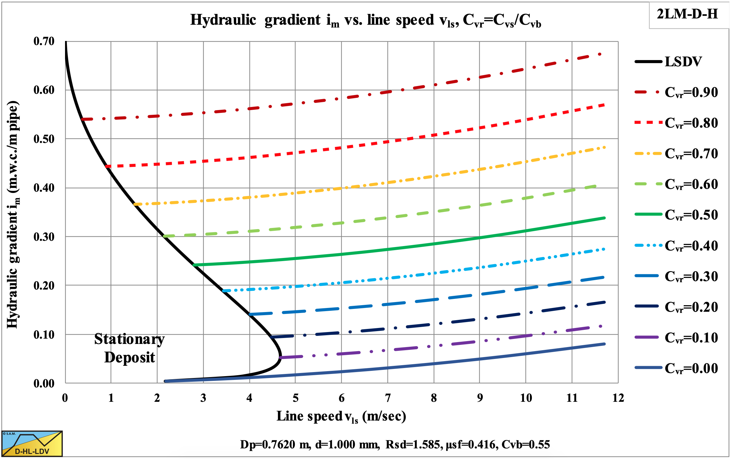
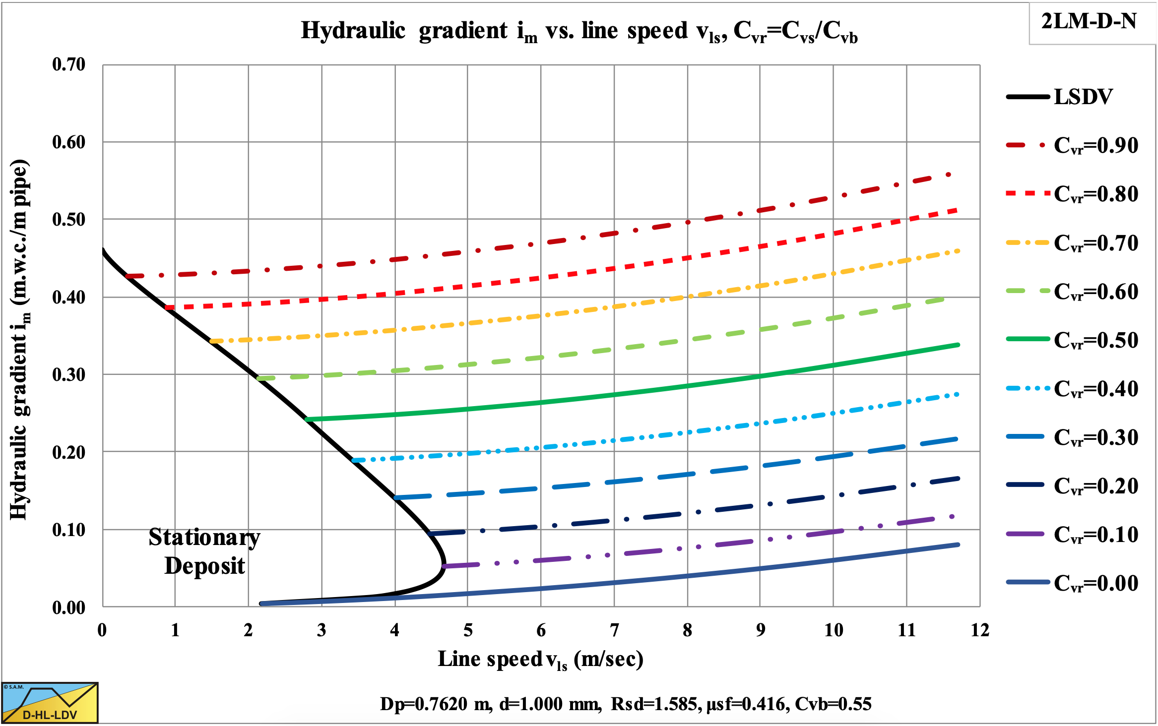
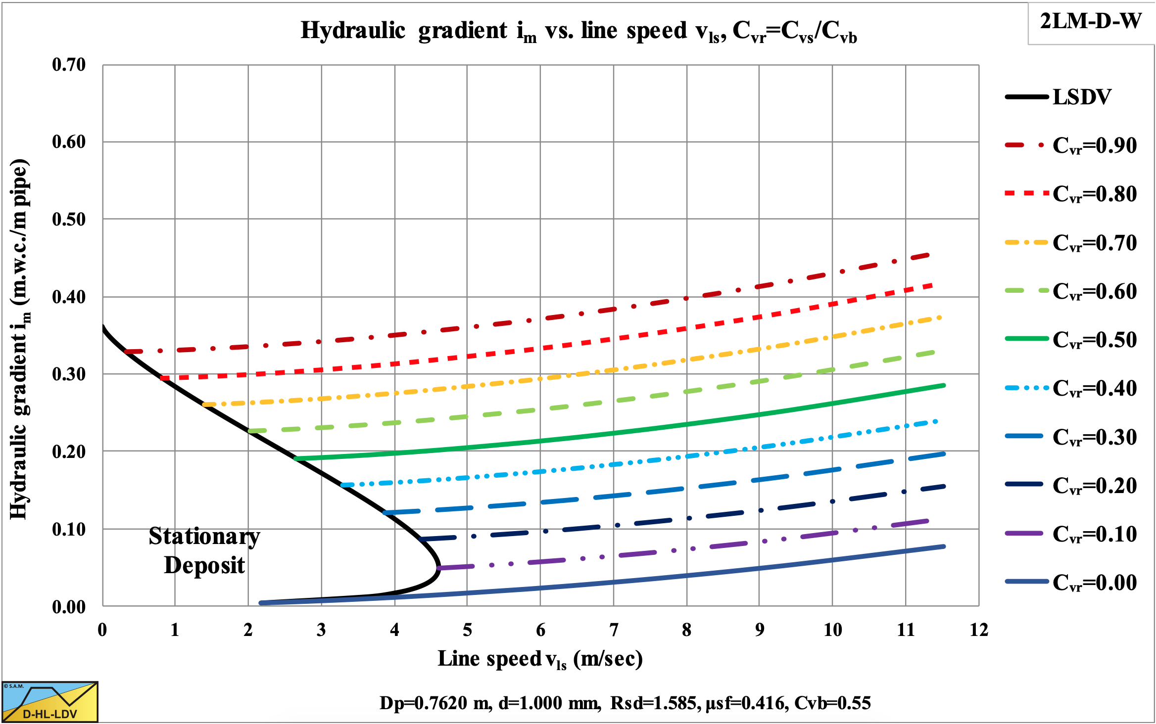
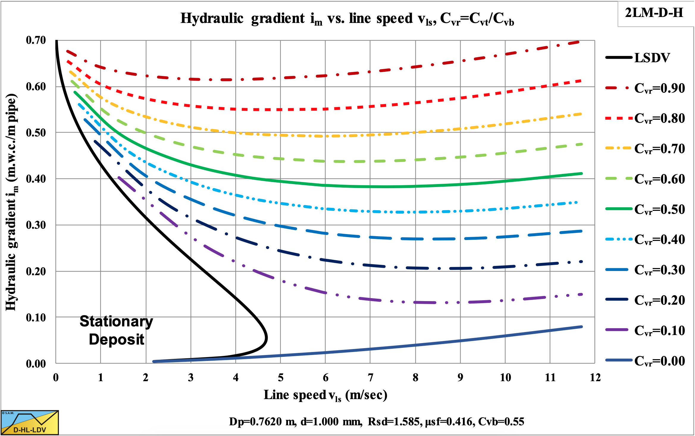
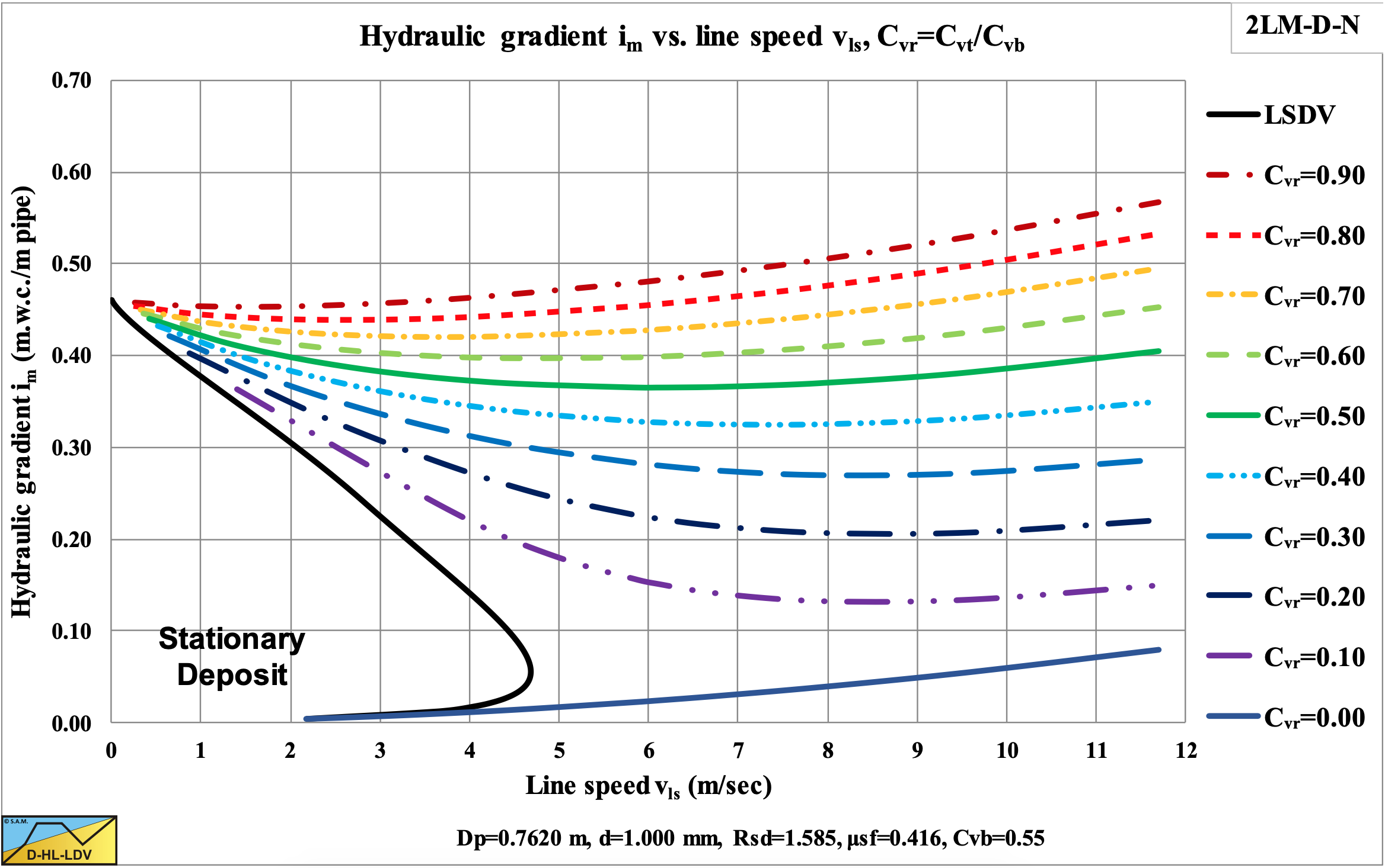
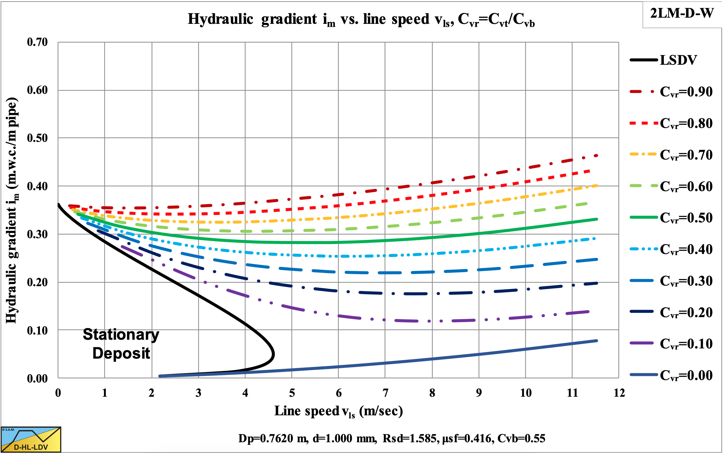
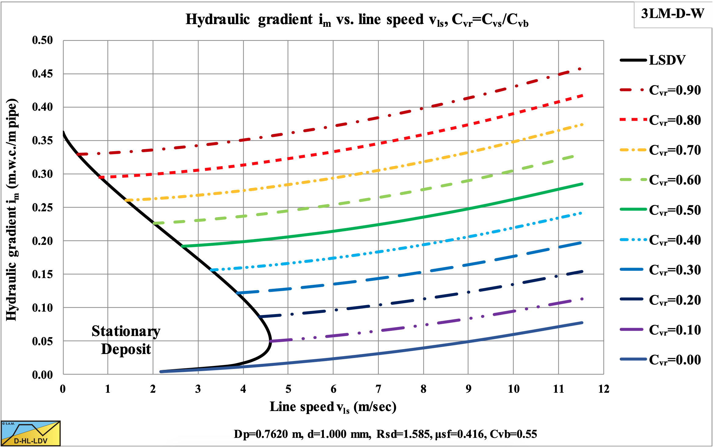
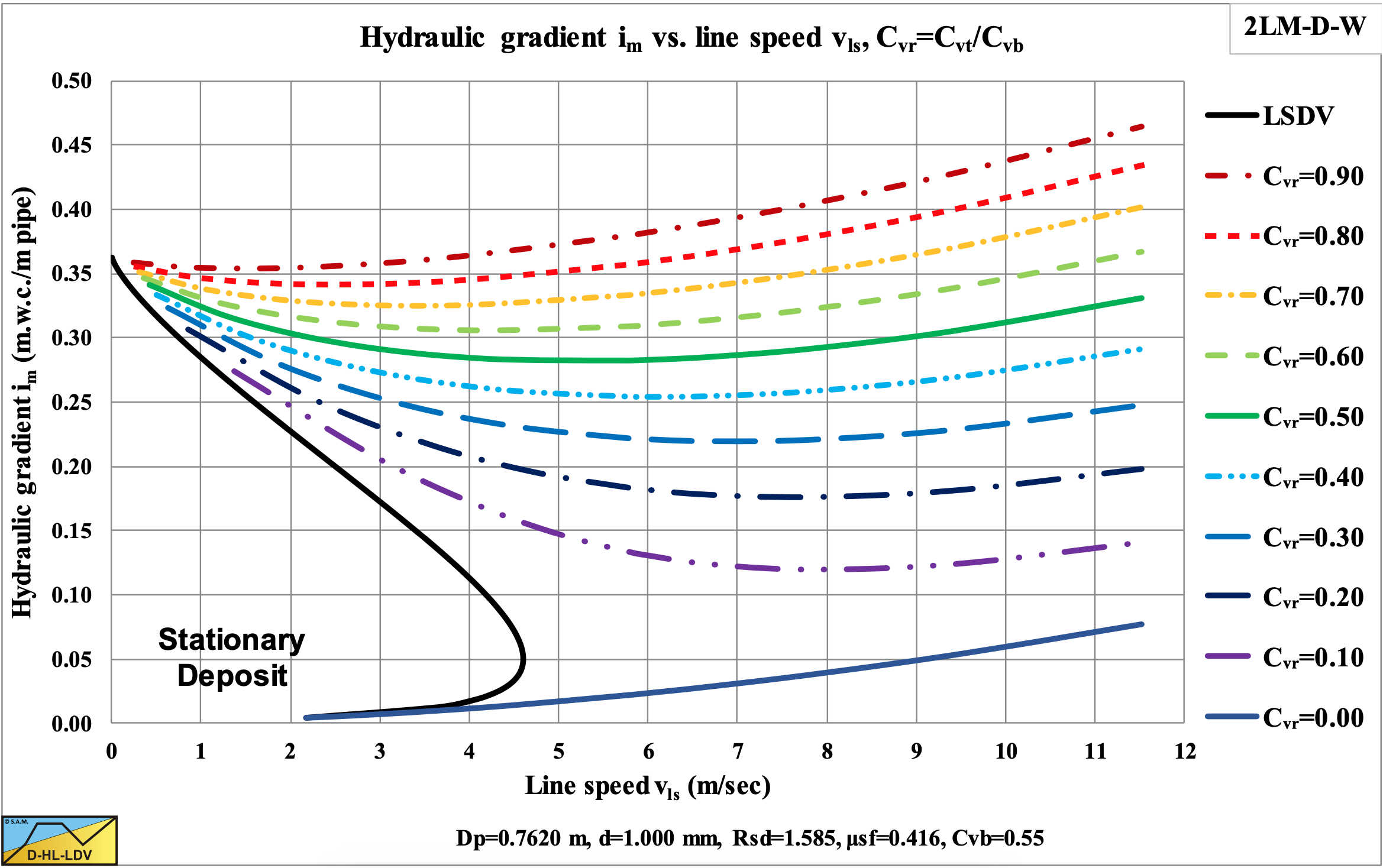
There are a number of approaches to determine the sliding friction force on a moving bed. These approaches are the original Wilson (1992) approach, based on the assumption that there is a hydrostatic pressure between the bed and the pipe wall. This assumes a pressure distribution as if the bed were a fluid, but the pipe wall friction based on the sliding coefficient of friction. The second approach assumes that the vertical component of the normal stress has to carry the weight of the bed. This approach is similar to the Wilson (1992) approach for pipes filled up to 50% with sand. Above 50% there is a significant difference between the two approaches, as the portion of the bed above the centerline of the pipe contributes weight but no friction. Another approach is the active/passive soil resistance approach, but it only gives solutions if the factor K=1, making it equivalent to the second approach. The third approach assumes that the sliding friction force is the result of the submerged weight of the bed times a sliding friction coefficient. In all 3 cases, solving the force equilibrium equations result in a Limit of Stationary Deposit Velocity curve (here defined as the velocity at which the bed starts sliding) and resistance curves based on constant spatial volumetric concentration. Figure 7.4-13, Figure 7.4-14 and Figure 7.4-15 give the hydraulic gradients for the 3 approaches for the constant spatial volumetric concentration curves. It is clear from these figures that the Wilson hydrostatic approach gives the highest hydraulic gradients (maximum factor 2 normal force to weight ratio), followed by the normal force carrying the weight approach (maximum factor 1.3 normal force to weight ratio), followed by the submerged weight approach (maximum factor 1 normal force to weight ratio).

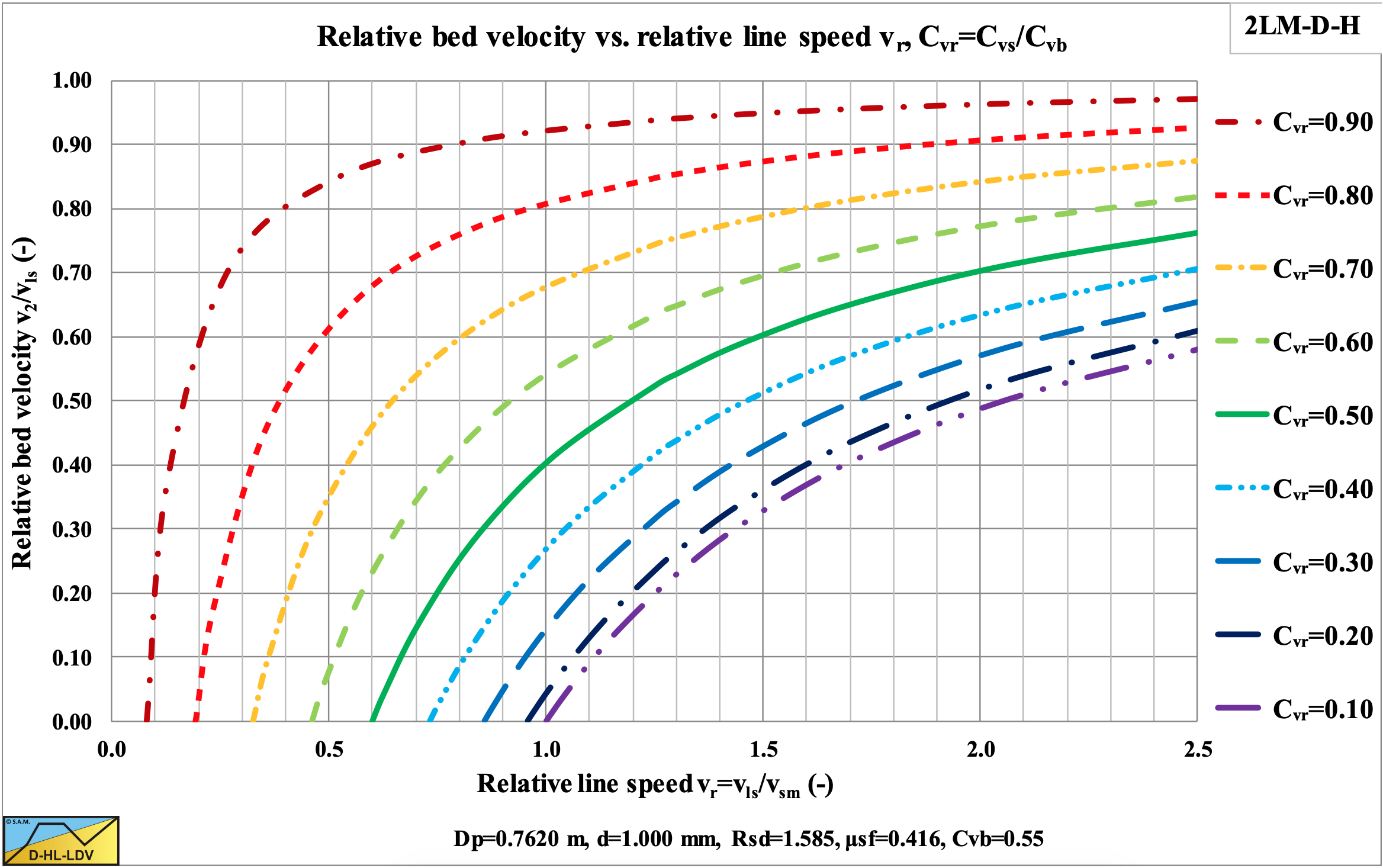
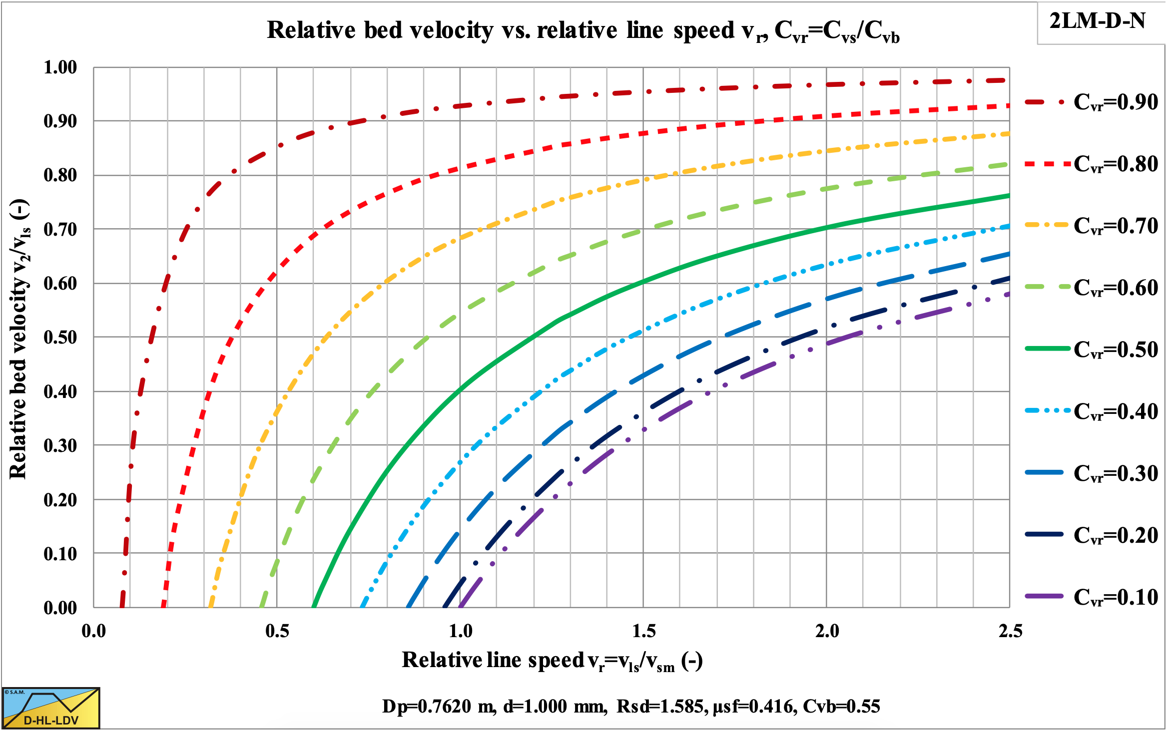
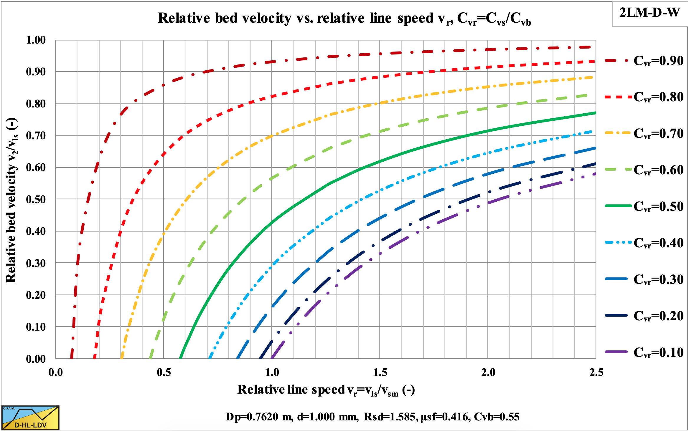
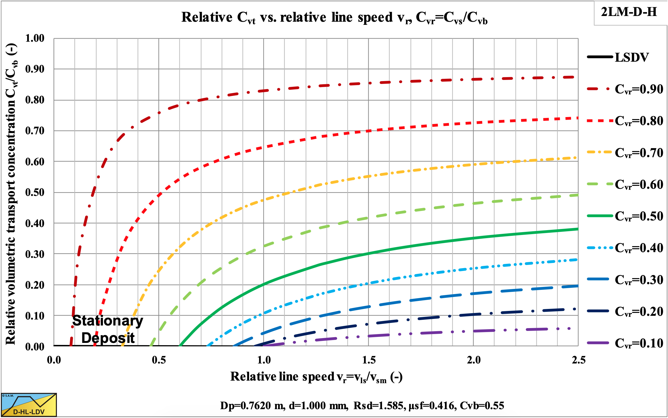
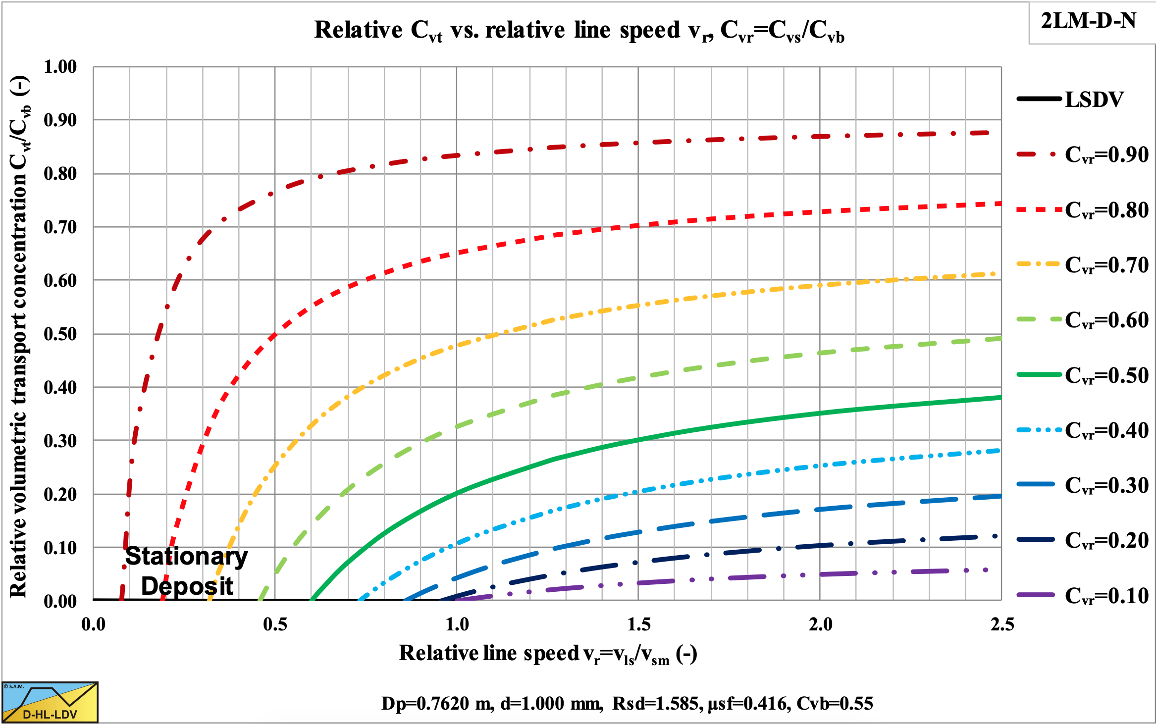
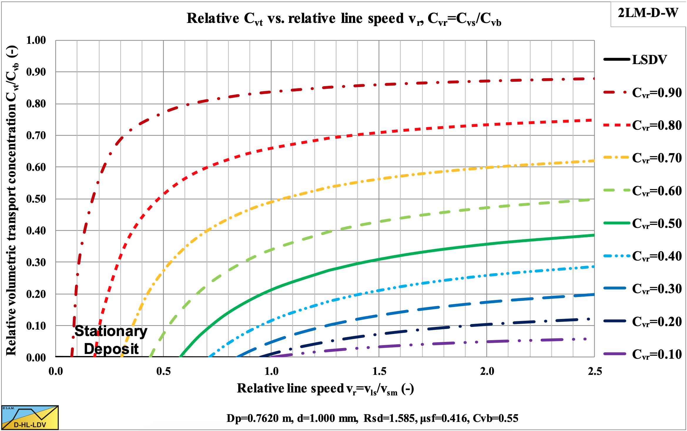
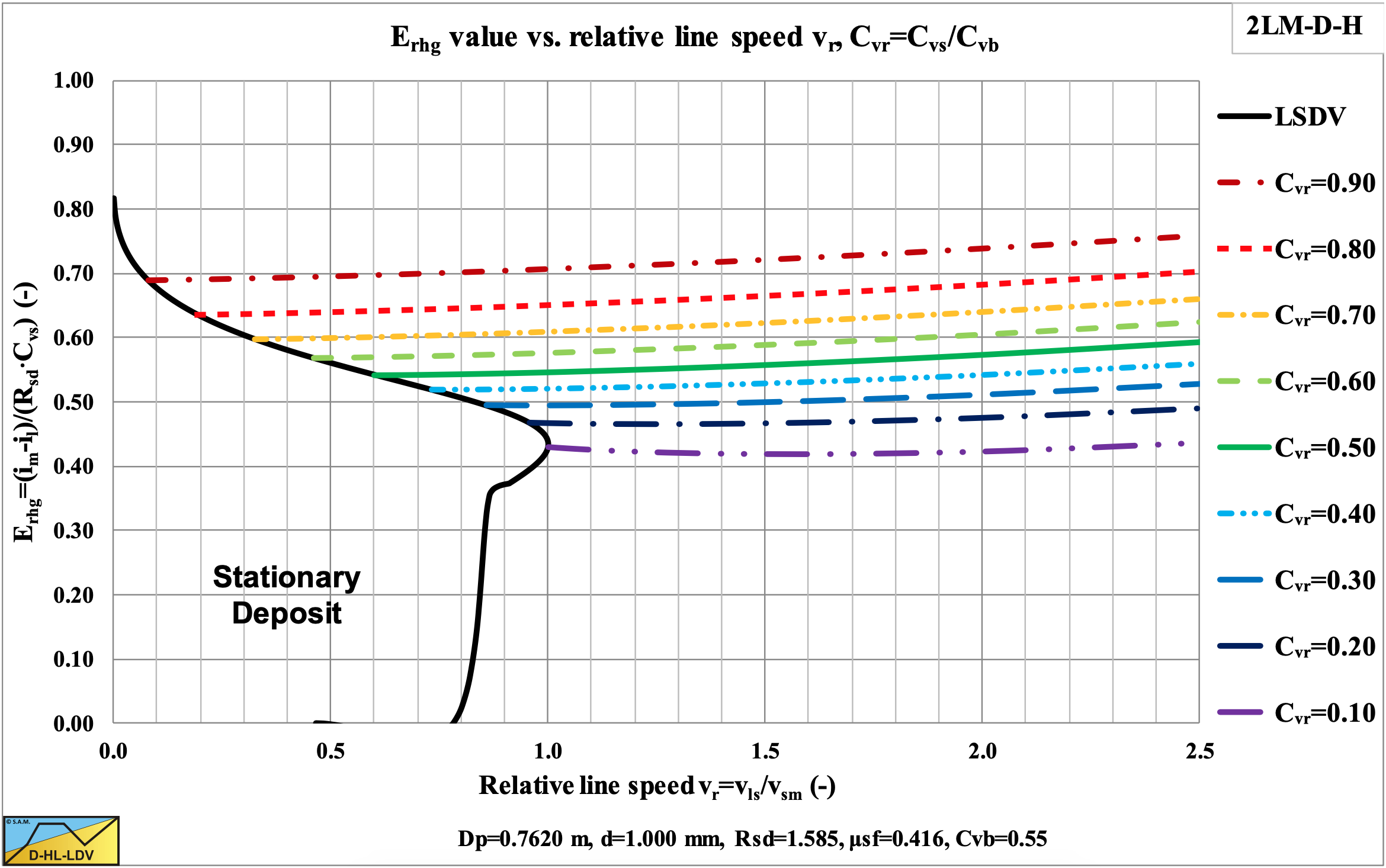
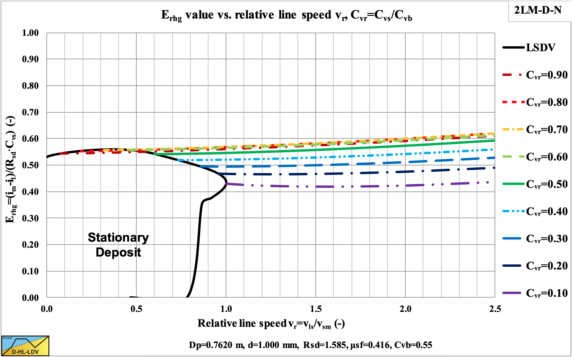
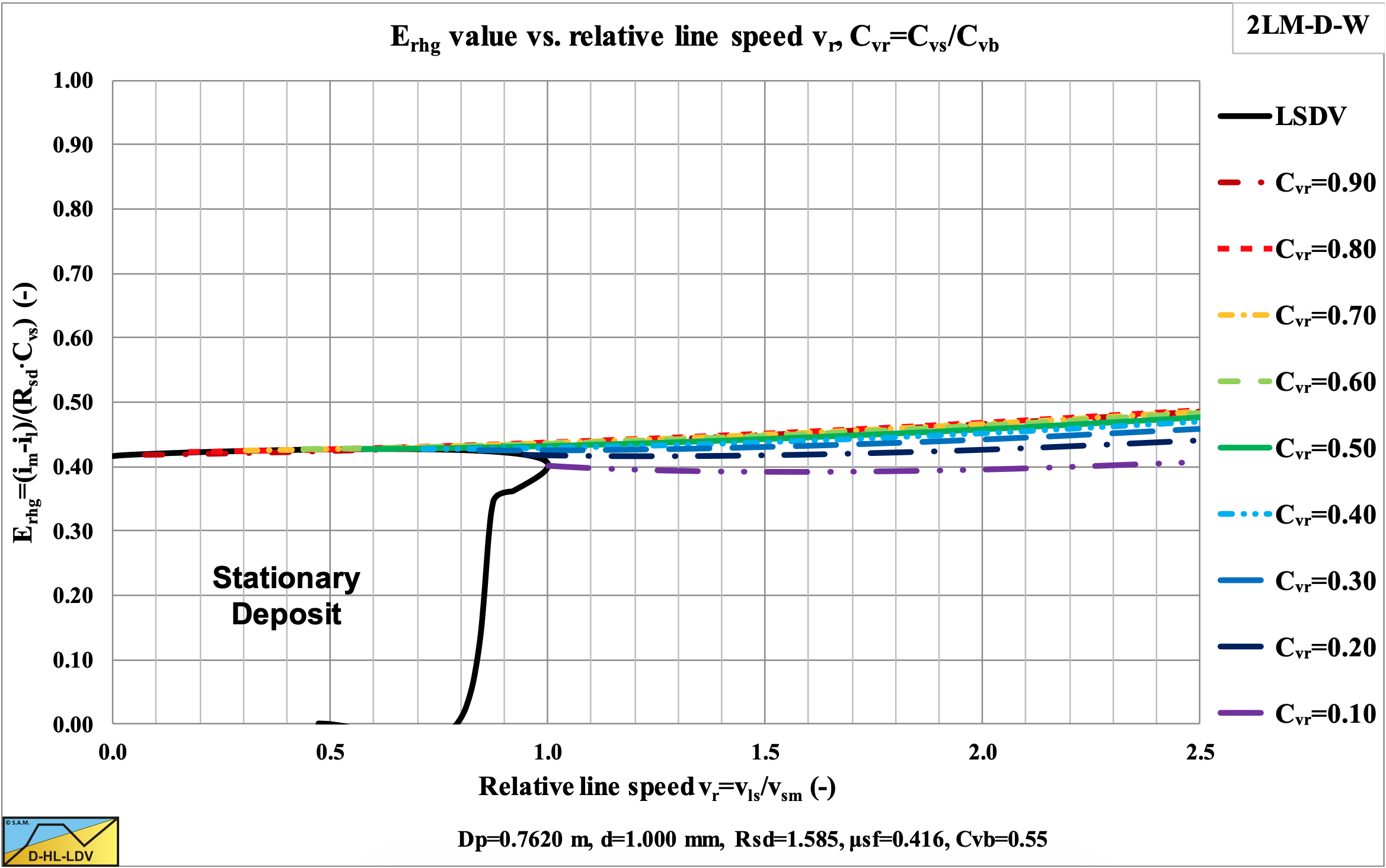
Based on the force equilibrium equations, the velocity of the sliding bed is determined and shown in Figure 7.4-16, Figure 7.4-17 and Figure 7.4-18 for the 3 approaches. Once the bed velocity is known, the delivered or transport concentration can be determined as is shown in Figure 7.4-19, Figure 7.4-20 and Figure 7.4-21. Now the transport concentrations are determined, hydraulic gradient curves for constant delivered or transport concentration can be determined by interpolation. Figure 7.4-22, Figure 7.4-23 and Figure 7.4-24 show the hydraulic gradients as a function of the delivered volumetric concentration. The curves never touch the Limit Deposit Velocity curves, since the delivered volumetric concentration is always zero on these curves, due to the assumption that there is only transport of particles if the bed is sliding. Figure 7.4-25, Figure 7.4-26 and Figure 7.4-27 show the relative excess hydraulic gradient (E_rhg) as a function of the spatial concentration. In the case of the submerged weight approach, this gives an almost constant E_rhg very close to the sliding friction coefficient μ_sf.

Now which approach to use? If there is only transport through a sliding bed, the second approach should be applied. The Wilson hydrostatic approach overestimates the total normal force between the bed and the pipe wall if the pipe is filled with more than 50% by the bed, by assuming both horizontal and vertical components of normal stress for the entire perimeter of the pipe filled by the bed. The normal stress carrying the weight of the bed approach gives a correct value for the normal force in this case. In practice however the pipe will never be filled more than 50% (this would cause plugging) so for practical applications the Wilson hydrostatic approach is suitable.

In practice however the sand transport will not only take place through a sliding bed only. If the velocity above the bed is high enough, sheet flow will occur. Sheet flow is a layer of fast moving particles on the top of the bed. The weight of these particles is still transferred to the bed and will contribute to the sliding friction force, but this layer of sheet flow will not result in sliding friction where it is in contact with the pipe wall. Of course, the higher the line speed, the thicker the layer of sheet flow (Miedema (2014)). This thicker layer of sheet flow implies a thinner bed and larger part of the solids that do not contribute to normal stresses on the wall, so the more the submerged weight approach is more valid.

Figure 7.4-13 to Figure 7.4-27 show a comparison between the 3 methods for the wall friction, using the Miedema & Matousek (2014) approach for the bed friction.

Figure 7.4-13: The hydraulic gradient i_m versus the line speed v_ls, C_vr=C_vs/C_vb. The hydrostatic Wilson approach.

Figure 7.4-14: The hydraulic gradient i_m versus the line speed v_ls, C_vr=C_vs/C_vb. The normal force carrying the weight approach.

Figure 7.4-15: The hydraulic gradient i_m versus the line speed v_ls, C_vr=C_vs/C_vb. The submerged weight approach.

Figure 7.4-16: The relative bed velocity v₂/v_ls versus the relative line speed v_r=v_ls/v_sm, C_vr=C_vs/C_vb. The hydrostatic Wilson approach.

Figure 7.4-17: The relative bed velocity v₂/v_ls versus the relative line speed v_r=v_ls/v_sm, C_vr=C_vs/C_vb. The normal force carrying the weight approach.

Figure 7.4-18: The relative bed velocity v₂/v_ls versus the relative line speed v_r=v_ls/v_sm, Cv_r=C_vs/C_vb. The submerged weight approach.

Figure 7.4-19: The relative volumetric transport concentration C_vt/C_vb versus the relative line speed v_r=v_ls/v_sm, C_vr=C_vs/C_vb. The hydrostatic Wilson approach.

Figure 7.4-20: The relative volumetric transport concentration C_vt/C_vb versus the relative line speed v_r=v_ls/v_sm, C_vr=C_vs/C_vb. The normal force carrying the weight approach.

Figure 7.4-21: The relative volumetric transport concentration C_vt/C_vb versus the relative line speed v_r=v_ls/v_sm, C_vr=C_vs/C_vb. The submerged weight approach.

Figure 7.4-22: The hydraulic gradient i_m versus the line speed v_ls, C_vr=C_vt/C_vb. The hydrostatic Wilson approach.

Figure 7.4-23: The hydraulic gradient i_m versus the line speed v_ls, C_vr=C_vt/C_vb. The normal force carrying the weight approach.

Figure 7.4-24: The hydraulic gradient im versus the line speed vls, Cvr=Cvt/Cvb. The submerged weight approach.

Figure 7.4-25: The relative excess hydraulic gradient E_rhg versus the relative line speed v_r=v_ls/v_sm, C_vs. The hydrostatic Wilson approach.

Figure 7.4-26: The relative excess hydraulic gradient E_rhg versus the relative line speed v_r=v_ls/v_sm, C_vs. The normal force carrying the weight approach.

Figure 7.4-27: The relative excess hydraulic gradient E_rhg versus the relative line speed v_r=v_ls/v_sm, C_vs. The submerged weight approach.

7.4.7 The 3 Layer Model

In the 2 layer model only the bed is transporting solids with the bed velocity. In the 3 layer model, the top of the bed is moving with a higher velocity as a sheet flow layer, so it is expected that the total transport of solids is larger in the 3LM compared to the 2LM.

Pugh & Wilson (1999) found a relation for the velocity at the top of the sheet flow layer with a stationary bed. This relation is modified here for a sliding bed, giving:

\[\ \mathrm{U}_{\mathrm{H}}=\gamma \cdot \mathrm{u}_{*}+\mathrm{v}_{2}=\gamma \cdot \sqrt{\frac{\lambda_{\mathrm{1} 2}}{\mathrm{8}}} \cdot\left(\mathrm{v}_{\mathrm{1}}-\mathrm{v}_{2}\right)+\mathrm{v}_{\mathrm{2}}=\mathrm{U}_{\mathrm{H} 0}+\mathrm{v}_{2} \quad\text{ with: }\quad \gamma=\mathrm{9 . 4}\]

The shear stress on the sheet flow layer has to be transferred to the bed by sliding friction. It is assumed that this sliding friction is related to the internal friction angle, giving for the thickness of the sheet flow layer:

\[\ \begin{array}{left}\mathrm{H}=\frac{\tau_{12}}{\rho_{\mathrm{l}} \cdot \mathrm{R}_{\mathrm{sd}} \cdot \mathrm{g} \cdot \mathrm{C}_{\mathrm{v} \mathrm{s}, \mathrm{s} \mathrm{f}} \cdot \tan (\varphi)} \approx \frac{\mathrm{2} \cdot \mathrm{\theta} \cdot \mathrm{d}}{\mathrm{C}_{\mathrm{v} \mathrm{b}} \cdot \mathrm{t a n}(\varphi)}\\
\text{With: }\quad \mathrm{C}_{\mathrm{v s}, \mathrm{s} \mathrm{f}}= \mathrm{0.4} \cdot \mathrm{C}_{\mathrm{v b}}-\mathrm{0 .5} \cdot \mathrm{C}_{\mathrm{v} \mathrm{b}} \quad\text{ and }\quad \tan (\varphi)=\mathrm{0 .5 7 7}\end{array}\]

Assuming a linear concentration distribution in the sheet flow layer, starting at the bed concentration C_vb at the bottom of the sheet flow layer and ending with a concentration of zero at the top of the sheet flow layer gives:

\[\ \mathrm{C_{v s}(z)=C_{v b} \cdot\left(\frac{H-z}{H}\right)}\]

With z the vertical coordinate starting at the bottom of the sheet flow layer and increasing going upwards. The velocity in the sheet flow layer is assumed to start with the bed velocity at the bottom and ends with U_H at the top following a power law according to:

\[\ \mathrm{U}(\mathrm{z})=\mathrm{U}_{\mathrm{H} 0} \cdot\left(\frac{\mathrm{z}}{\mathrm{H}}\right)^{\mathrm{n}}+\mathrm{v}_{\mathrm{2}}\]

The cross section of the sheet flow layer, reduced to the bed concentration C_vb is, assuming the average spatial sheet flow layer concentration is 50% of the bed concentration:

\[\ \Delta \mathrm{A}_{\mathrm{s f}}=\mathrm{H} \cdot \mathrm{O}_{12} \cdot \frac{\mathrm{C}_{\mathrm{v s}, \mathrm{s f}}}{\mathrm{C}_{\mathrm{v b}}} \approx \frac{\mathrm{H} \cdot \mathrm{O}_{12}}{\mathrm{2}}\]

The total amount of solids transported Q_s is the amount transported in the remaining bed Q₂ + the amount transported in the sheet flow layer Q₁₂. The amount of solids transported in the bed is, corrected for the solids in the sheet flow layer:

\[\ \mathrm{Q}_{2}=\mathrm{v}_{2} \cdot\left(\mathrm{A}_{2}-\Delta \mathrm{A}_{\mathrm{s f}}\right) \cdot \mathrm{C}_{\mathrm{v b}}\]

The transport of solids in the sheet flow layer can now be determined by integration of the spatial concentration profile times the velocity profile in the sheet flow layer:

\[\ \mathrm{Q}_{12}=\mathrm{O}_{12} \cdot \int_{\mathrm{0}}^{\mathrm{H}} \mathrm{C}_{\mathrm{v s}}(\mathrm{z}) \cdot \mathrm{U}(\mathrm{z}) \cdot \mathrm{d z}=\mathrm{O}_{\mathrm{1 2}} \cdot \int_{\mathrm{0}}^{\mathrm{H}} \mathrm{C}_{\mathrm{v b}} \cdot\left(\frac{\mathrm{H}-\mathrm{z}}{\mathrm{H}}\right) \cdot\left(\mathrm{U}_{\mathrm{H} 0} \cdot\left(\frac{\mathrm{z}}{\mathrm{H}}\right)^{\mathrm{n}}+\mathrm{v}_{2}\right) \cdot \mathrm{d z}\]

\[\ \mathrm{Q}_{12}=\mathrm{O}_{\mathrm{1} 2} \cdot \mathrm{C}_{\mathrm{v b}} \cdot\left(\mathrm{v}_{\mathrm{2}} \cdot \int_{\mathrm{0}}^{\mathrm{H}}\left(\frac{\mathrm{H}-\mathrm{z}}{\mathrm{H}}\right) \cdot \mathrm{d z}+\mathrm{U}_{\mathrm{H} 0} \cdot \int_{\mathrm{0}}^{\mathrm{H}}\left(\frac{\mathrm{H}-\mathrm{z}}{\mathrm{H}}\right) \cdot\left(\frac{\mathrm{z}}{\mathrm{H}}\right)^{\mathrm{n}} \cdot \mathrm{d z}\right)\]

This can be rewritten to:

\[\ \mathrm{Q}_{12}=\mathrm{O}_{12} \cdot \mathrm{C}_{\mathrm{v b}} \cdot\left(\mathrm{v}_{2} \cdot \int_{\mathrm{0}}^{\mathrm{H}}\left(\mathrm{1}-\frac{\mathrm{z}}{\mathrm{H}}\right) \cdot \mathrm{d z}+\mathrm{U}_{\mathrm{H} 0} \cdot \int_{\mathrm{0}}^{\mathrm{H}}\left(\left(\frac{\mathrm{z}}{\mathrm{H}}\right)^{\mathrm{n}}-\left(\frac{\mathrm{z}}{\mathrm{H}}\right)^{\mathrm{n}+1}\right) \cdot \mathrm{d z}\right)\]

Integration gives:

\[\ \mathrm{Q}_{12}={\mathrm{O}}_{12} \cdot{\mathrm{C}}_{\mathrm{v b}} \cdot\left({\mathrm{v}}_{2} \cdot\left(\mathrm{z}-\frac{\mathrm{1}}{2} \cdot \mathrm{z}^{2}\right)+\mathrm{U}_{\mathrm{H} 0} \cdot \mathrm{H} \cdot\left(\frac{\mathrm{1}}{(\mathrm{n}+\mathrm{1})} \cdot\left(\frac{\mathrm{z}}{\mathrm{H}}\right)^{\mathrm{n}+1}-\frac{\mathrm{1}}{(\mathrm{n}+\mathrm{2})} \cdot\left(\frac{\mathrm{z}}{\mathrm{H}}\right)^{\mathrm{n}+2}\right)\right)_{0}^{\mathrm{H}}\]

With integration from zero to the thickness of the sheet flow layer this gives:

\[\ \mathrm{Q_{12}=H \cdot O_{12} \cdot C_{v b}} \cdot\left(\frac{\mathrm{v_{2}}}{2}+\frac{\mathrm{U_{H 0}}}{\mathrm{(n+1) \cdot(n+2)}}\right)\]

The total flow of solids equals the bed flow plus the sheet flow, which can be estimated by:

\[\ \mathrm{Q}_{\mathrm{s}}=\mathrm{Q}_{2}+\mathrm{Q}_{12}=\mathrm{v}_{2} \cdot\left(\mathrm{A}_{2}-\Delta \mathrm{A}_{\mathrm{s f}}\right) \cdot \mathrm{C}_{\mathrm{v b}}+\left(\mathrm{v}_{2}+\frac{\mathrm{2} \cdot \mathrm{U}_{\mathrm{H} 0}}{(\mathrm{n}+\mathrm{1}) \cdot(\mathrm{n}+\mathrm{2})}\right) \cdot \Delta \mathrm{A}_{\mathrm{s f}} \cdot \mathrm{C}_{\mathrm{v} \mathrm{b}}\]

The delivered volumetric concentration equals the solids flow divided by the total flow:

\[\ \mathrm{C}_{\mathrm{v t}}=\frac{\mathrm{Q}_{\mathrm{s}}}{\mathrm{v}_{\mathrm{l} \mathrm{s}} \cdot \mathrm{A}_{\mathrm{p}}}\]

The above equations describe a relatively simple method to add sheet flow to the 2LM (2 layer model). This is possible because an explicit relation for the Darcy-Weisbach friction factor has been developed. Analyses of the above equations shows that the sheet flow concentration is not really important. Choosing a smaller sheet flow concentration results in a thicker sheet flow layer, but does not influence the velocity at the top of the sheet flow layer. A smaller sheet flow concentration does also not influence the reduced sheet flow cross-section and thus it does not influence the resulting delivered volumetric concentration.

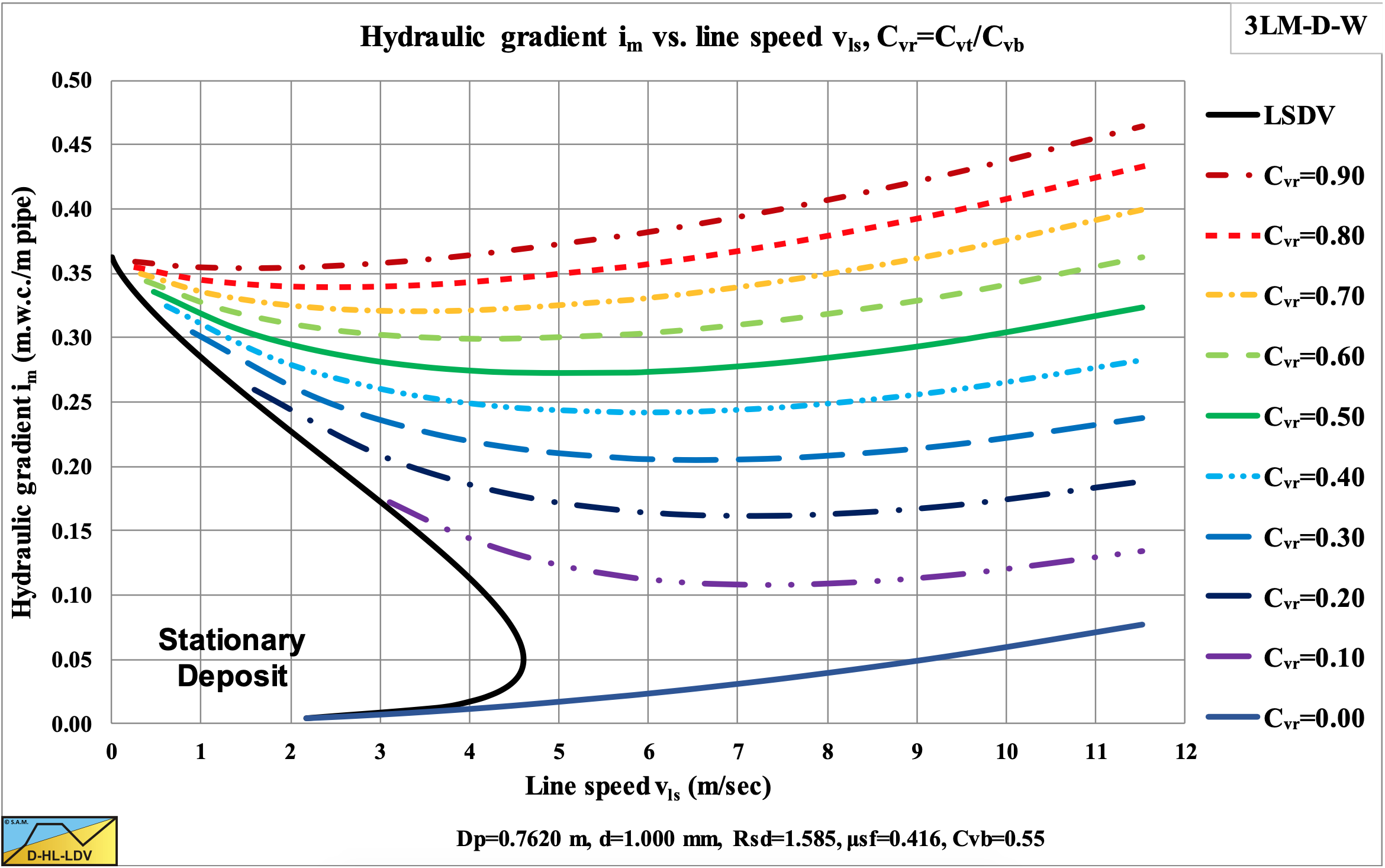
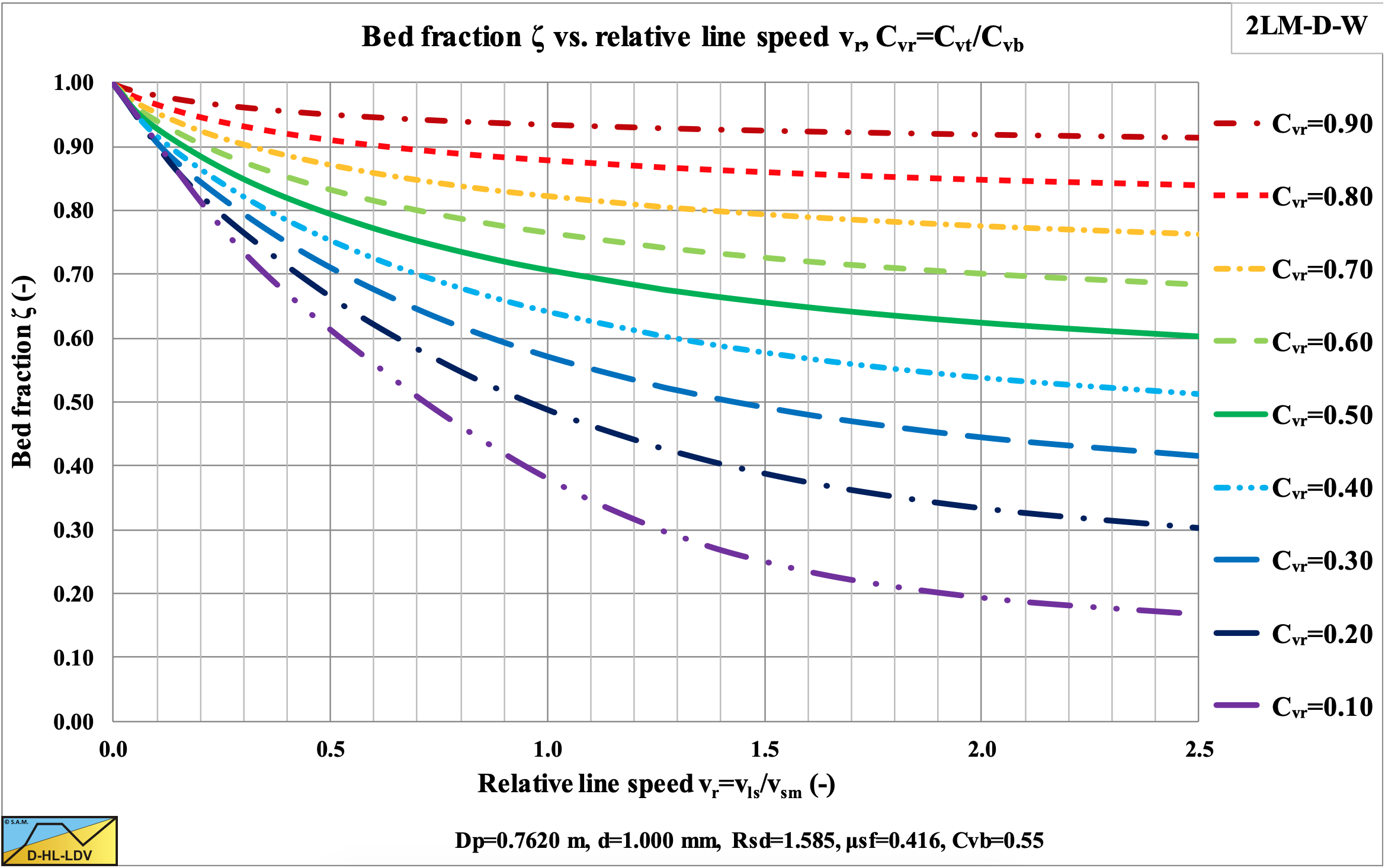
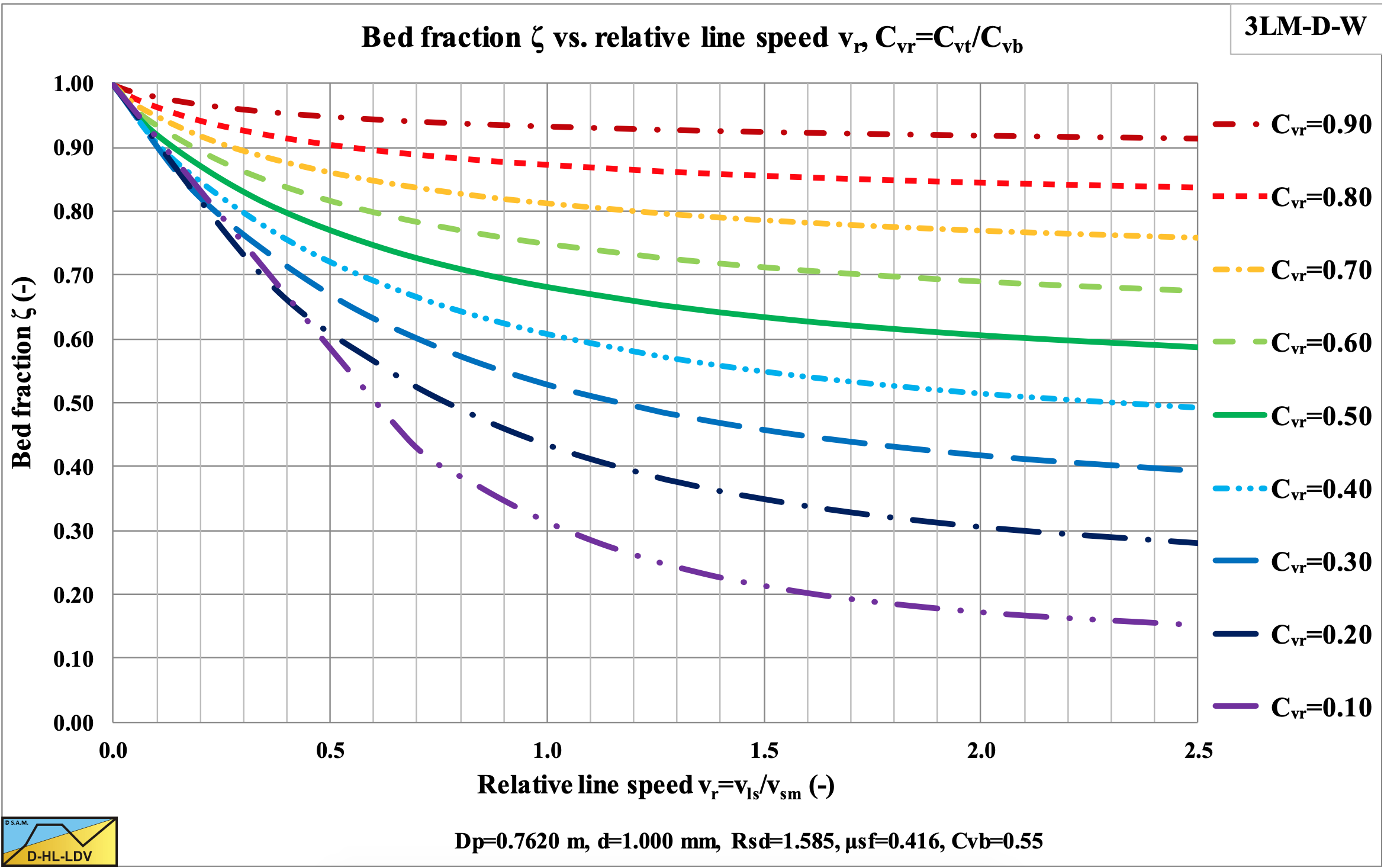
Figure 7.4-28 to Figure 7.4-35 show a comparison between the 2LM and 3LM approach using the Miedema & Matousek (2014) method for the bed friction and the weight approach of Miedema & Ramsdell (2014) for the wall friction.

This model gives good predictions up to a certain line speed. First of all when the line speed is increasing, a part of the solids will be in suspension above the bed or above the sheet flow layer. This part of the solids is not taken into account in the model. This part will reduce the bed fraction, reduce the slip ratio and reduce the hydraulic gradient. Secondly, if the thickness of the sheet flow layer approaches the bed height, the whole bed will become sheet flow and the assumption of having sliding friction between the bed and the pipe wall will no longer be valid. This will also result in a strong decrease of the slip ratio and the hydraulic gradient. In fact there will no longer be a sliding bed and a heterogeneous model should be used.

Figure 7.4-36 shows a comparison between the 3LM and the DHLLDV Framework regarding the slip ratio. At very low line speeds both models match close, but above a certain line speed, the DHLLDV Framework shows a strong reduction of the slip ratio, due to suspension and a dissolving bed. The conclusion is, that the 3LM model is suitable for very low line speeds, but not for line speeds close to the LDV, the line speed where the bed has been dissolved completely. Extending the 3LM with suspension above the sheet flow layer might improve the model.

The total flow of solids can be related to the Shields parameter, which is:

\[\ \theta=\frac{\tau_{12}}{\rho_{\mathrm{l}} \cdot \mathrm{R_{\mathrm{sd}}} \cdot \mathrm{g} \cdot \mathrm{d}}=\frac{\mathrm{u}_{*}^{2}}{\mathrm{R}_{\mathrm{sd}} \cdot \mathrm{g} \cdot \mathrm{d}} \quad\text{ or }\quad \mathrm{u}_{*}=\sqrt{\theta \cdot \mathrm{R}_{\mathrm{sd}} \cdot \mathrm{g} \cdot \mathrm{d}}\]

The velocity on top of the sheet flow layer can now be written as:

\[\ \begin{array}{left} \mathrm{U}_{\mathrm{H}}=\gamma \cdot \mathrm{u}_{*}+\mathrm{v}_{2}=\gamma \cdot \sqrt{\boldsymbol{\theta} \cdot \mathrm{R}_{\mathrm{s} \mathrm{d}} \cdot \mathrm{g} \cdot \mathrm{d}}+\mathrm{v}_{\mathrm{2}}\\
\text{ With :} \quad \mathrm{U}_{\mathrm{H} \mathrm{0}}=\gamma \cdot \sqrt{\boldsymbol{\theta} \cdot \mathrm{R}_{\mathrm{s} \mathrm{d}} \cdot \mathrm{g} \cdot \mathrm{d}}\end{array}\]

The total flow of solids equals the bed flow plus the sheet flow, which can be estimated by after substitution of the sheet flow layer cross section and the velocity on top of the sheet flow layer:

\[\ \mathrm{Q_{s}}=\mathrm{v_{2} \cdot\left(A_{2}-\frac{H \cdot O_{12}}{2}\right) \cdot C_{v b}+\left(v_{2}+\frac{2 \cdot \gamma \cdot \sqrt{\theta \cdot R_{s d} \cdot g \cdot d}}{(n+1) \cdot(n+2)}\right) \cdot \frac{H \cdot O_{12}}{2} \cdot C_{v b}}\]

Substituting the equation for the sheet flow layer thickness gives:

\[\ \begin{array}{left} \mathrm{Q_{s}=v_{2} \cdot\left(A_{2}-\frac{\theta \cdot d \cdot O_{12}}{C_{v b} \cdot \tan (\varphi)}\right) \cdot C_{v b}+\left(v_{2}+\frac{2 \cdot \gamma \cdot \sqrt{\theta \cdot R_{s d} \cdot g \cdot d}}{(n+1) \cdot(n+2)}\right) \cdot \frac{\theta \cdot d \cdot O_{12}}{C_{v b} \cdot \tan (\varphi)} \cdot C_{v b}}\\
\mathrm{Q_{s}=v_{2} \cdot A_{2} \cdot C_{v b}+\frac{2 \cdot \gamma \cdot \sqrt{\theta \cdot R_{s d} \cdot g \cdot d}}{(n+1) \cdot(n+2)} \cdot \frac{\theta \cdot d \cdot O_{12}}{C_{v b} \cdot \tan (\varphi)} \cdot C_{v b}}\\
\mathrm{Q_{s}=v_{2} \cdot A_{2} \cdot C_{v b}+\frac{2 \cdot \gamma}{(n+1) \cdot(n+2) \cdot \tan (\varphi)} \cdot d \cdot \sqrt{R_{s d} \cdot g \cdot d} \cdot O_{12} \cdot \theta^{3 / 2}}\end{array}\]

The first term on the right hand side shows the solids transport assuming that all solids in the pipe are transported in the bed with cross section A₂ with a velocity v₂. The second term on the right hand side shows the additional solids transport, because the velocity in the sheet flow layer is higher than the bed velocity. The latter is not the total solids transport in the sheet flow layer, just the additional solids transport compared with the case where there is no sheet flow layer. In the case of a stationary bed, v₂=0, this gives:

\[\ \mathrm{Q_{s}=\frac{2 \cdot \gamma}{(n+1) \cdot(n+2) \cdot \tan (\varphi)} \cdot d \cdot \sqrt{R_{s d} \cdot g \cdot d} \cdot O_{12} \cdot \theta^{3/2}}\]

This can be written as a transport equation similar to the Meyer-Peter Muller (1948) (MPM) equation, giving the solods transport rate per unit of width of the bed in a dimensionless form:

\[\ \frac{\mathrm{Q}_{\mathrm{s}}}{\mathrm{d} \cdot \sqrt{\mathrm{R}_{\mathrm{s d}} \cdot \mathrm{g} \cdot \mathrm{d}}{ \cdot \mathrm{O}_{\mathrm{1} 2}}}=\frac{\mathrm{2} \cdot \gamma}{(\mathrm{n}+\mathrm{1}) \cdot(\mathrm{n}+\mathrm{2}) \cdot \mathrm{\operatorname { tan } ( \varphi )}}{ \cdot \mathrm{\theta}^{3/2}=\mathrm{\alpha} \cdot \mathrm{\theta}^{\beta}}\]

The original MPM equation includes the critical Shields parameter, giving:

\[\ \frac{\mathrm{Q}_{\mathrm{s}}}{\mathrm{d} \cdot \sqrt{\mathrm{R}_{\mathrm{s} \mathrm{d}} \cdot \mathrm{g} \cdot \mathrm{d}} \cdot \mathrm{O}_{\mathrm{1 2}}}=\mathrm{\alpha} \cdot\left(\mathrm{\theta}-\mathrm{\theta}_{\mathrm{c r}}\right)^{\beta} \quad\text{ with: }\quad \alpha=\mathrm{8} \quad\text{ and }\quad \beta=\mathrm{1 . 5}\]

For high values of the Shields parameter, both equations behave the same. With n=1 and tan(φ)=0.6, the theoretical equation gives α=5.22. With n=1 and tan(φ)=0.4, the theoretical equation gives α=8. With n=0.537 and tan(φ)=0.6, the theoretical equation also gives α=8. So both equations give results in the same range.

Figure 7.4-28: The hydraulic gradient i_m versus the line speed v_ls, C_vr=C_vs/C_vb. The submerged weight approach, without sheet flow.

Figure 7.4-29: The hydraulic gradient i_m versus the line speed v_ls, C_vr=C_vs/C_vb. The submerged weight approach, with sheet flow.

The sheet flow at the top of the bed does not influence the hydraulic gradient in the constant C_vs graphs, since in both the 2LM and the 3LM use the same equation is used for the bed shear stress. In the constant C_vt graphs however there is a difference because the transport concentration is influenced by the sheet flow. Also the slip and the bed fraction are influenced by the sheet flow.

Figure 7.4-30: The hydraulic gradient im versus the line speed v_ls, C_vr=C_vt/C_vb. The submerged weight approach, without sheet flow.

Figure 7.4-31: The hydraulic gradient im versus the line speed v_ls, C_vr=C_vt/C_vb. The submerged weight approach, with sheet flow.

Figure 7.4-32: The slip factor (1-ξ) resulting from the 2 layer model.

Figure 7.4-33: The slip factor (1-ξ) resulting from the 3 layer model.

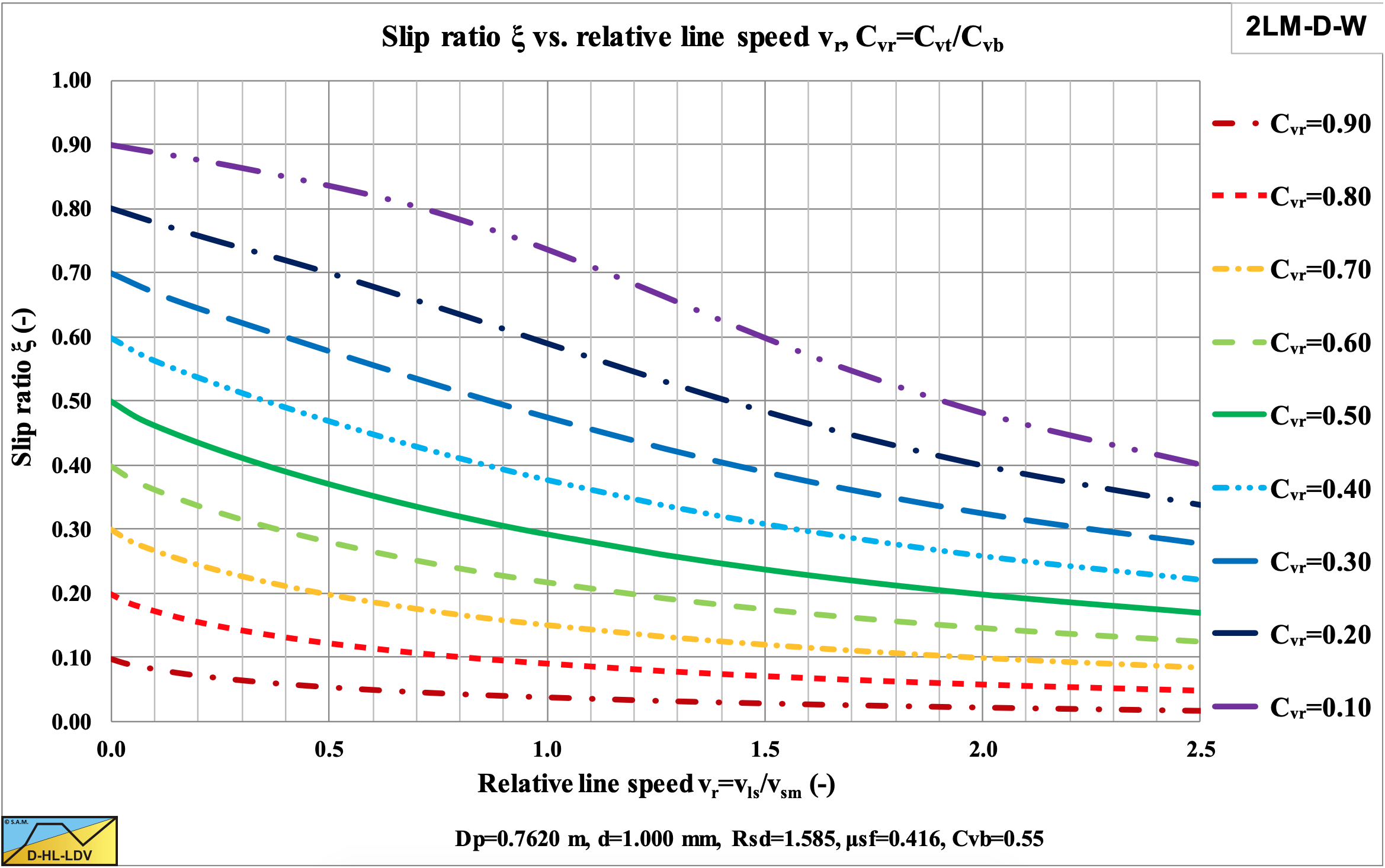
The slip ratio of the 3 layer model is smaller than the slip factor of the 2 layer model, which is expected. This means that the 3 layer model results in less slip, which is to be expected.

Figure 7.4-34: The bed fraction ζ resulting from the 2 layer model.

Figure 7.4-35: The bed fraction ζ resulting from the 3 layer model.

Figure 7.4-36: A comparison of the slip ratio, 3LM versus DHLLDV.

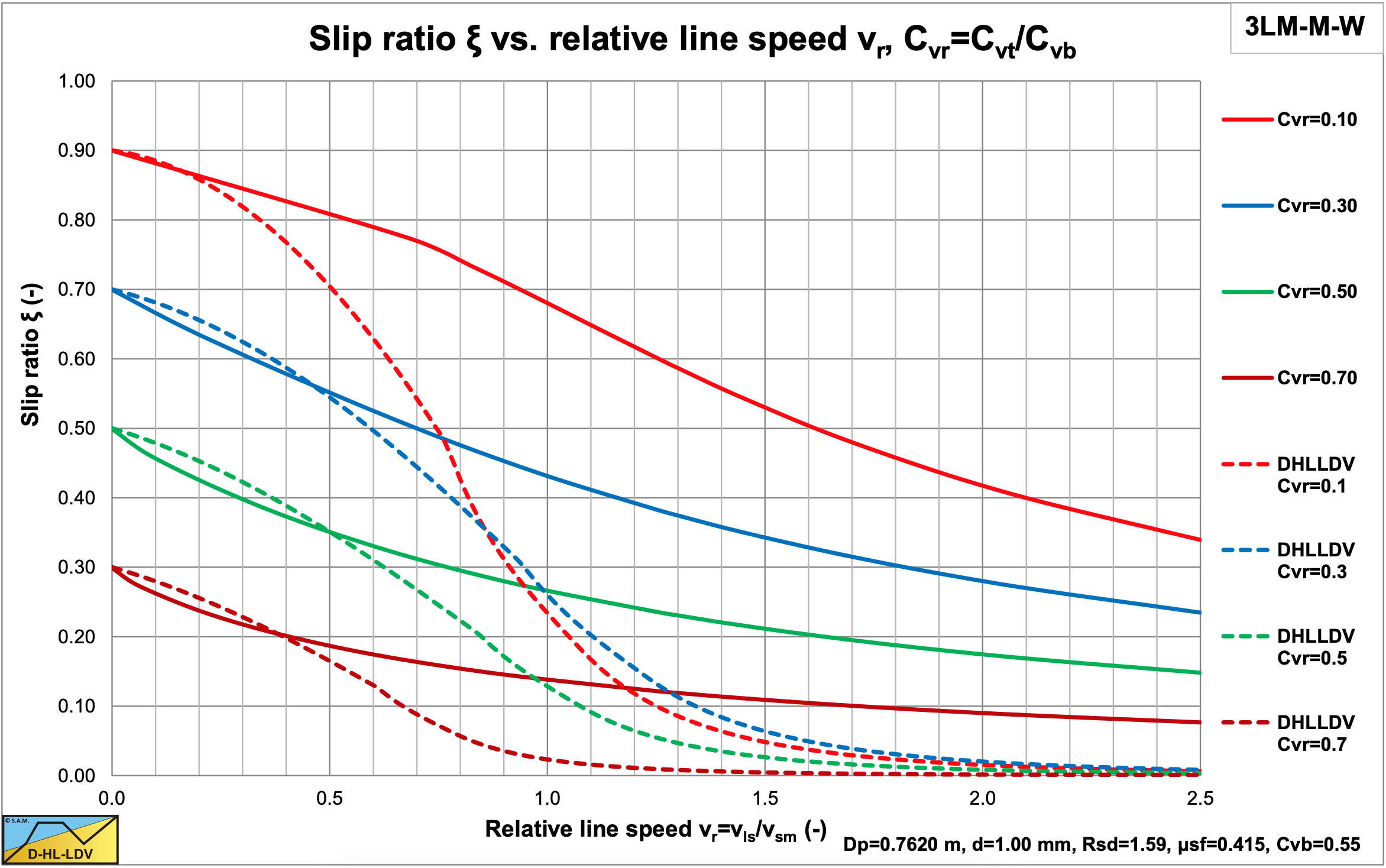
The slip ratio from Figure 7.4-33 can be estimated by the following empirical equation:

\[\ \begin{array}{left}\mathrm{C}_{\mathrm{v r}}=\frac{\mathrm{C}_{\mathrm{v t}}}{\mathrm{C}_{\mathrm{v} \mathrm{b}}} \quad\text{ and }\quad \alpha=\mathrm{0 . 5 8} \cdot \mathrm{C}_{\mathrm{v r}}^{-\mathrm{0} .42}\\ \frac{1}{1-\xi_{\mathrm{v}_{\mathrm{ls}, \mathrm{lsdv}}}}=\mathrm{C}_{\mathrm{vr}}^{-0.5}\\ \xi=\left(1-\mathrm{C}_{\mathrm{v r}}\right) \cdot \mathrm{e}^{\left(-\left(0.83+\frac{\mu_{\mathrm{sf}}}{4}+\left(\mathrm{c}_{\mathrm{vr}}-\mathrm{0 . 5 - 0 . 0 7 5 . \mathrm { D } _ { \mathrm { p } }}\right)^{2}+0.025 \cdot \mathrm{D}_{\mathrm{p}}\right) \cdot \mathrm{D}_{\mathrm{p}}^{0.025} \cdot\left(\frac{\mathrm{v}_{\mathrm{ls}}}{\mathrm{v}_{\mathrm{ls}, \mathrm{lsdv}}}\right)^{\alpha} \cdot \mathrm{C}_{\mathrm{vr}}^{0.65} \cdot\left(\frac{\mathrm{R}_{\mathrm{sd}}}{1.585}\right)^{0.1}\right)}\end{array}\]

This equation has been developed based on the 3 layer approach, but is considered empirical. With additional simulations or modifications of the fundamental model, this equation may change in the future.

7.4.8 Nomenclature Sliding Bed Regime

Ap	Cross section pipe	m^2
A1	Cross section above bed	m^2
A2 ​​​​​​​	Cross section bed	m^2
Asf	Cross section sheet flow layer	m^2
Cvb	Volumetric bed concentration	-
Cvs	Spatial volumetric concentration	-
Cvs,1 ​​​​​​​	Spatial volumetric concentration upper layer	-
Cvs,2 ​​​​​​​	Spatial volumetric concentration lower layer, bed	-
Cvs,sf	Average spatial concentration in sheet flow layer	-
Cvt	Delivered (transport) volumetric concentration	-
Cvr	Relative volumetric concentration	-
d	Particle diameter	m
Dp	Pipe diameter	m
Erhg	Relative excess hydraulic gradient	-
Fn	Normal force	kN
Ft	Tangent force	kN
Fw	Weight of bed	kN
Fsf	Sliding friction force	kN
Fh	Horizontal force	kN
Fh,n	Component horizontal force normal to pipe wall	kN
Fh,t	Component horizontal force tangent to pipe wall	kN
Fv	Vertical force	kN
Fv,n	Component vertical force normal to pipe wall	kN
Fv,t	Component vertical force tangent to pipe wall	kN
hb	Bed height above point on the pipe wall	m
H	Thickness sheet flow layer	m
g	Gravitational constant 9.81 m/s^2	m/s^2
il ​​​​​​​	Hydraulic gradient pure liquid	m/m
im ​​​​​​​	Hydraulic gradient mixture	m/m
iplug	Hydraulic gradient plug flow	m/m
K	Failure factor, ratio horizontal stress to vertical stress	-
Ka	Factor of active failure	-
Kp	Factor of passive failure	-
ΔL	Length of pipe section	m
n	Power of velocity distribution in sheet flow layer	-
Op	Circumference pipe	m
O1 ​​​​​​​	Circumference pipe above bed	m
O2 ​​​​​​​	Circumference pipe in bed	m
O12	Width of bed	m
Δpl ​​​​​​​	Head loss pure liquid	kPa
Δpm ​​​​​​​	Head loss mixture	kPa
Qs	Total amount of solids transported by volume	m^3/s
Q2	Amount of solids transported in the bed	m^3/s
Q12	Amount of solids transported in the sheet flow layer	m^3/s
Rsd	Relative submerged density	-
R	Pipe radius	m
u*	Friction velocity	m/s
UH	Velocity at the top of the sheet flow layer	m/s
UH0	Velocity at the top of the sheet flow layer with fixed bed	m/s
vls	Line speed	m/s
vr	Relative line speed	-
vsm	Maximum Limit of Stationary Deposit Velocity	m/s
v1	Velocity above bed	m/s
v1,m	Mean velocity above bed, upper layer	m/s
v2	Velocity bed	m/s
v2,m	Mean velocity bed, lower layer	m/s
yb	Height of bed	m
z	Vertical coordinate in sheet flow layer	m
α	Angle of position in bed	rad
α	Factor MPM equation	-
β	Bed angle	rad
β	Power MPM equation	-
φ	Angle of internal friction	rad
\(\ \gamma\)	Wilson factor velocity at top of sheet flow layer	-
ρl	Density carrier liquid	ton/m^3
θ	Shields parameter	-
θc	Critical Shields parameter	-
λ12	Darcy-Weisbach friction factor on the bed	-
\(\ \tau_{12}\)	Shear stress bed-liquid	kPa
\(\ \tau_{\mathrm{sf}}\)	Shear stress due to sliding friction	kPa
\(\ \tau_{\mathrm{t}}\)	Shear stress in bed tangent to pipe wall	kPa
μsf	Sliding friction coefficient	-
μsf,e	Effective or mobilized sliding friction coefficient	-
σn	Normal stress	kPa
σh	Horizontal stress	kPa
σv	Vertical stress	kPa
ζ	Bed fraction	-
ξ	Slip ratio	-