9.1: Introduction

In order to compare the different models discussed, criteria have to be defined. Models may be considered as black boxes, only considering the input and the output, which is possible for all models. Models can be distinguished in fully empirical, semi empirical and mechanistic/fundamental. Models can be compared based on their origin, the range of the parameters used in the experiments.

The main parameters of influence on the head losses are the pipe diameter D_p, the particle diameter d or the whole PSD, the relative submerged density of the solids R_sd, the spatial or delivered volumetric concentration C_vs or C_vt and the range of operational line speeds (related to the pipe diameter). The sliding friction coefficient μ_sf also plays a role, but only for large particles with a sliding bed in the range of operational parameters.

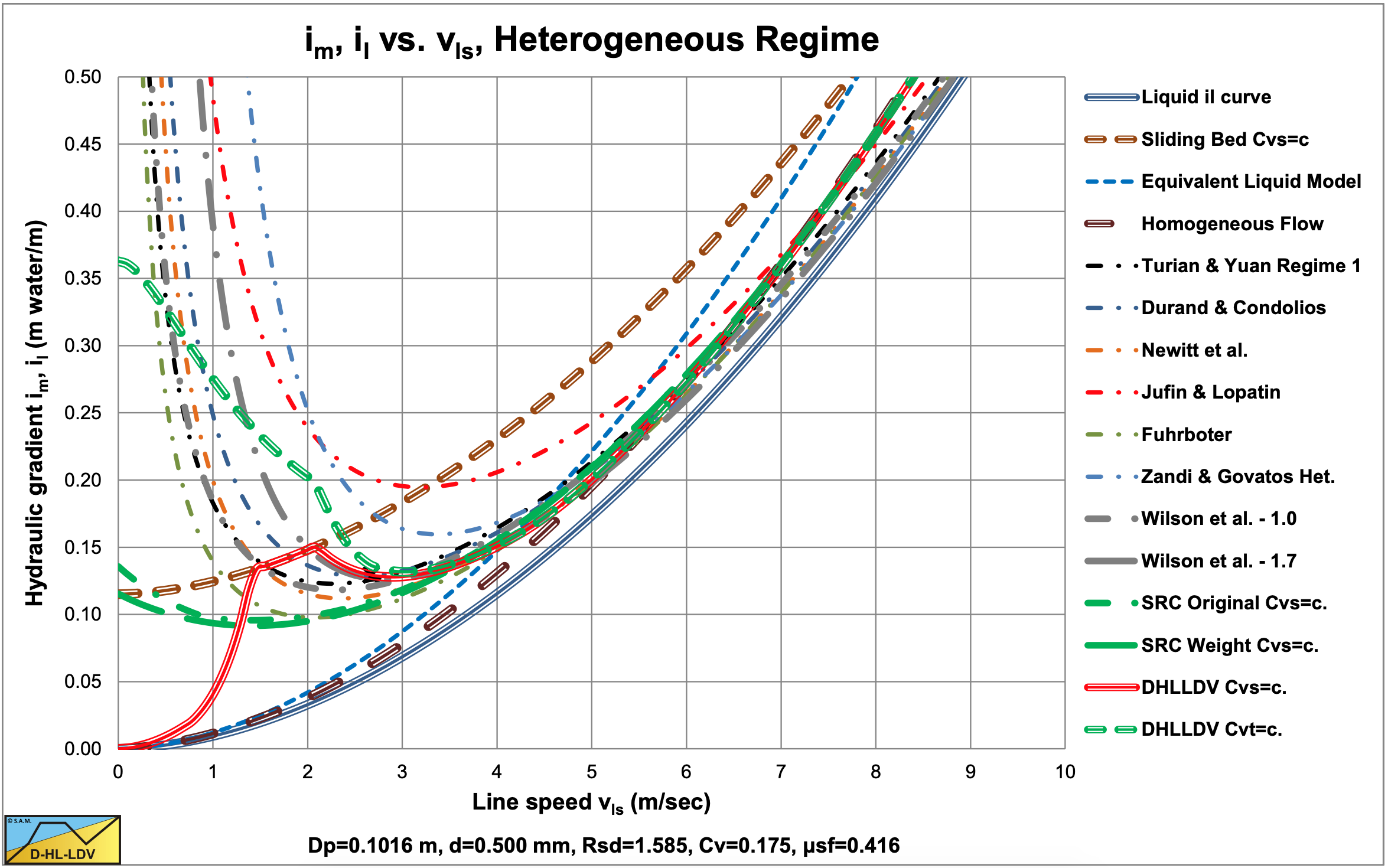
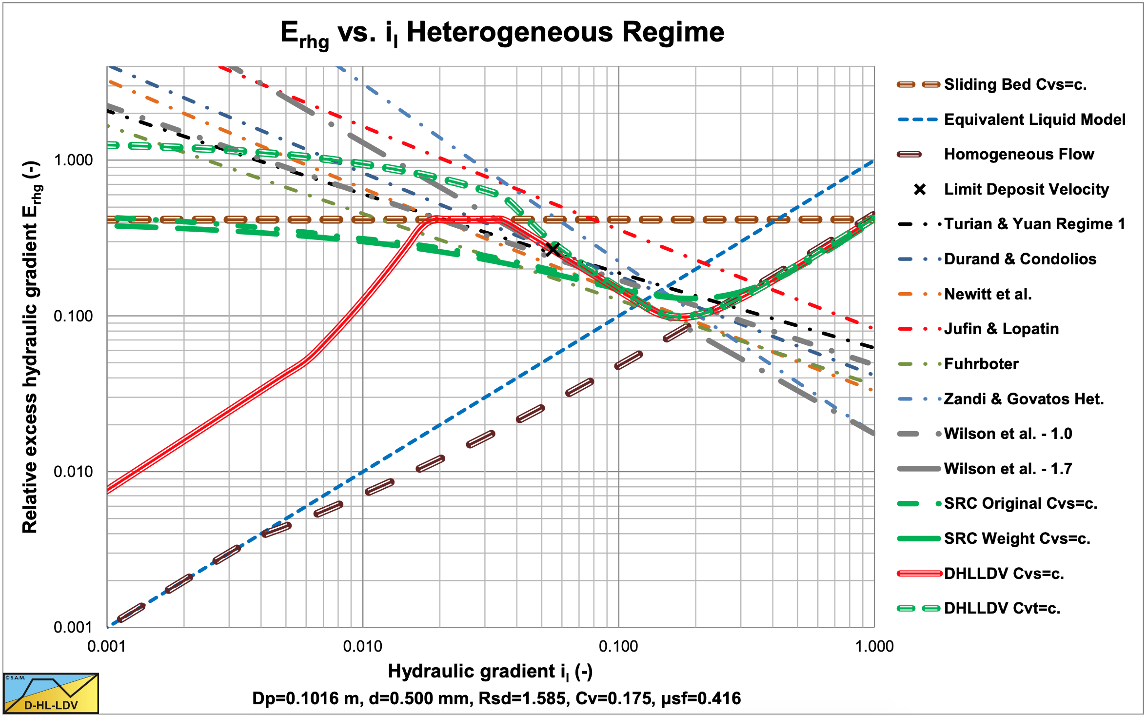
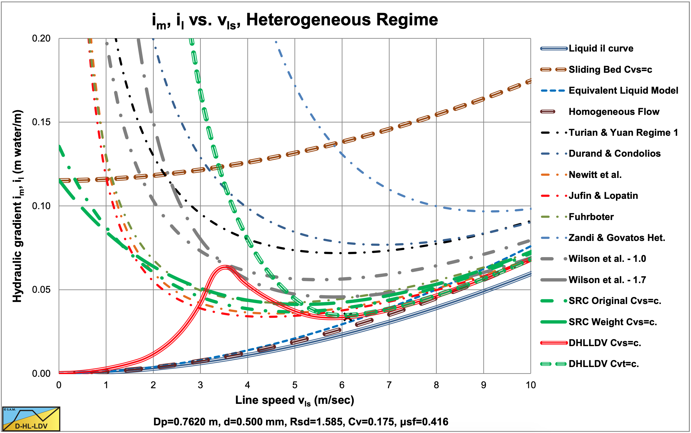
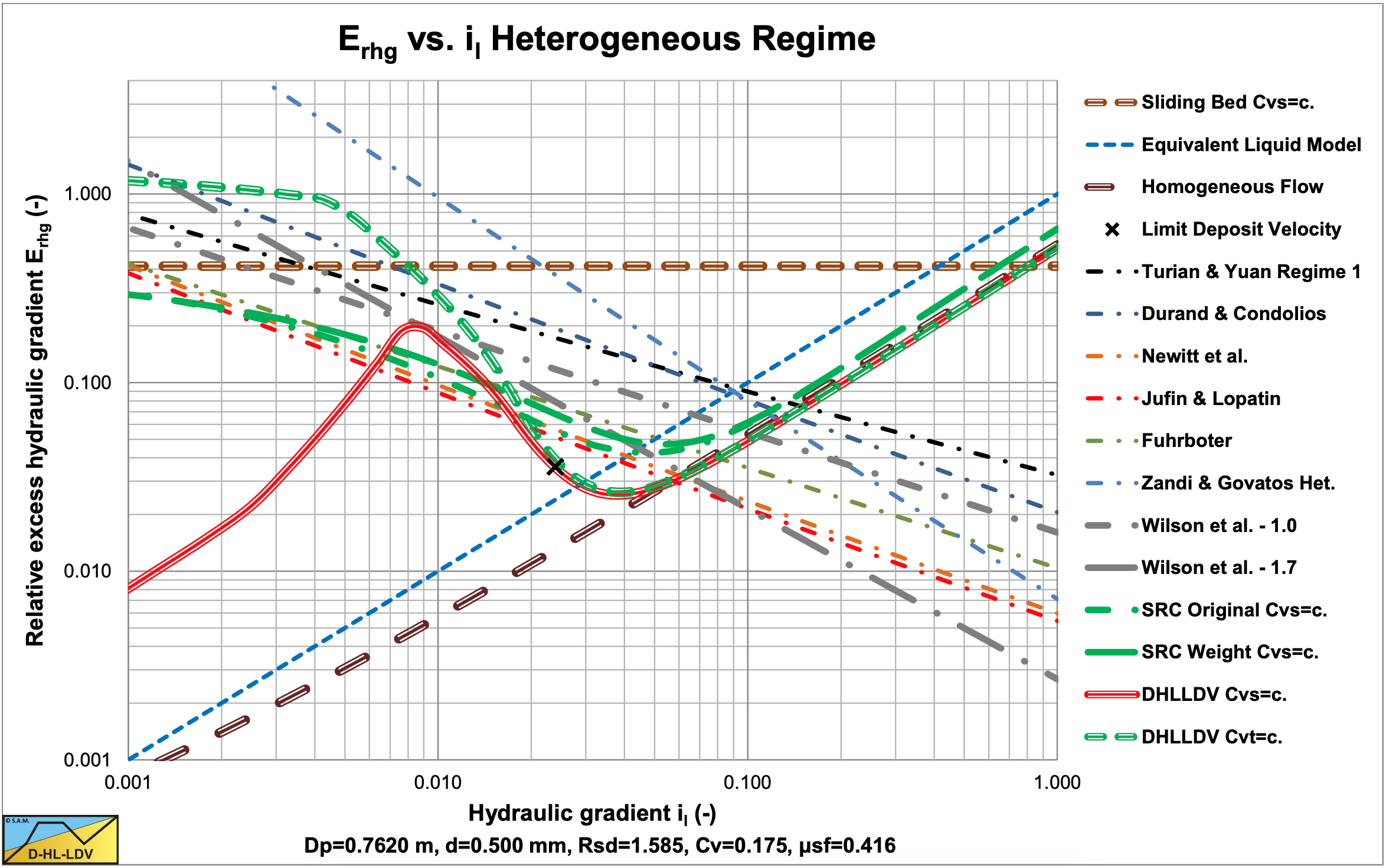
So basically there are 4 main parameters, the pipe diameter, the particle diameter, the relative submerged density and the volumetric concentration. If for each of these parameters 10 values are used, D_p from 0.0254 m to 1 m, d from 0.1 mm to 10 mm, R_sd from 0.1 to 10 and C_vs or C_vt from 0.01 to 0.5, 10,000 possibilities are found for the comparison. Figure 9.1-1 and Figure 9.1-3 show such a comparison of 22 models in a hydraulic gradient i_m versus line speed v_ls graph. There would be 10,000 graphs required to give a good overview of all possible combinations. Figure 9.1-2 and Figure 9.1-4 show the relative excess hydraulic gradient E_rhg versus the pure liquid hydraulic gradient i_l. Since the relative excess hydraulic gradient equals the mixture hydraulic gradient minus the pure liquid hydraulic gradient, which is the solids effect, divided by the relative submerged density and the volumetric concentration, an almost dimensionless graph is created. Almost dimensionless because most models are proportional to the volumetric concentration and more or less proportional to the relative submerged density. Using a concentration of about 20% and the relative submerged density of sand and gravel already limits the number of graphs to 100. However this is still to many.
The remaining parameters are the pipe diameter and the particle diameter. With the knowledge that the ELM often used for the homogeneous regime and most models for the heterogeneous regime are proportional or close to proportional to both the volumetric concentration and the relative submerged density, the conclusion can be drawn that the intersection point of these two regimes (the transition velocity) is almost independent of the volumetric concentration and the relative submerged density. With the knowledge that this transition velocity is often in the range of operational line speeds for medium sands, this transition velocity seems to be a good indicator for a model. For each particles diameter and each model a transition velocity is found, resulting in a graph with the transition velocity versus the particle diameter. The only parameter left is thus the pipe diameter. The following graphs (Figure 9.2-5, Figure 9.2-6, Figure 9.2-7, Figure 9.2-8 Figure 9.2-9, Figure 9.2-10, Figure 9.2-11, Figure 9.2-12, Figure 9.2-13, Figure 9.2-14, Figure 9.2-15, Figure 9.2-16, Figure 9.2-17 and Figure 9.2-18) have a dimensionless vertical axis by dividing the transition line speed by the maximum transition line speed occurring in one of the 11 models. Although most models are proportional with the volumetric concentration, a few are not. This is why the graphs are given for volumetric concentrations of 5% and 30%, limiting the number of graphs to 14 for sands and gravels.

In order to understand the graphs the following variables are given:

The hydraulic gradient of the pure liquid i_l is:

\[\ \mathrm{i}_{\mathrm{l}}=\frac{\lambda_{\mathrm{l}} \cdot \mathrm{v}_{\mathrm{l s}}^{2}}{\mathrm{2 \cdot g \cdot D_{p}}}\]

The relative excess hydraulic gradient E_rhg is, for spatial and delivered concentrations:

\[\ \mathrm{E}_{\mathrm{rhg}}=\frac{\mathrm{i}_{\mathrm{m}}-\mathrm{i}_{\mathrm{l}}}{\mathrm{R}_{\mathrm{sd}} \cdot \mathrm{C}_{\mathrm{vs}}} \quad\text{ or }\quad \mathrm{E}_{\mathrm{rhg}}=\frac{\mathrm{i}_{\mathrm{m}}-\mathrm{i}_{\mathrm{l}}}{\mathrm{R}_{\mathrm{sd}} \cdot \mathrm{C}_{\mathrm{vt}}}\]

The hydraulic gradient in the homogeneous regime, according to ELM i_m so without corrections, is:

\[\ \mathrm{i}_{\mathrm{m}}=\mathrm{i}_{\mathrm{l}} \cdot\left(\mathrm{1}+\mathrm{R}_{\mathrm{s d}} \cdot \mathrm{C}_{\mathrm{v s}}\right) \quad\text{ and }\quad \mathrm{E}_{\mathrm{r h g}}=\frac{\mathrm{i}_{\mathrm{m}}-\mathrm{i}_{\mathrm{l}}}{\mathrm{R}_{\mathrm{s d}} \cdot \mathrm{C}_{\mathrm{v s}}}=\mathrm{i}_{\mathrm{l}}\]

Figure 9.1-1: Comparison of 22 models in a i_m-v_ls graph in a D_p=0.1016 m (4 inch) pipe.

Figure 9.1-2: Comparison of 22 models in a E_rhg-i_l graph in a D_p=0.1016 m (4 inch) pipe.

Figure 9.1-3: Comparison of 22 models in a i_m-v_ls graph in a D_p=0.762 m (30 inch) pipe.

Figure 9.1-4: Comparison of 22 models in a E_rhg-i_l graph in a D_p=0.762 m (30 inch) pipe.