9.2: The Transition Velocity Heterogeneous-Homogeneous

9.2.1 Considerations

The theoretical transition velocity between the heterogeneous regime and the homogeneous regime gives a good indication of the excess pressure losses due to the solids. For normal dredging applications with large diameter pipes and rather high line speeds, this transition velocity will be at a line speed higher than the Limit Deposit Velocity and will often be near the operating range of the dredging operations. The excess head losses are in some way proportional to this transition velocity. For a D_p=0.15 m diameter pipe most models match pretty well, due to the fact that most experiments are carried out in small diameter pipes and the models are fitted to the experiments. Although the different models may have a different approach, the resulting equations go through the same cloud of data points. Since there are numerous fit lines of numerous researchers it is impossible to cover them all, so a choice is made to compare Durand & Condolios (1952), Newitt et al. (1955), Fuhrboter (1961), Jufin & Lopatin (1966), Zandi & Govatos (1967), Turian & Yuan (1977), the SRC model and Wilson et al. (1992) with the DHLLDV Framework as developed here, Miedema & Ramsdell (2013).

9.2.2 The DHLLDV Framework

This theoretical transition velocity can be determined by making the relative excess pressure contributions of the heterogeneous regime and the homogeneous regime equal. This is possible if transition effects are omitted and the basic equations are applied.

The hydraulic gradient in the homogeneous regime, according to ELM so without corrections, is:

\[\ \mathrm{i}_{\mathrm{m}}=\mathrm{i}_{\mathrm{l}} \cdot\left(\mathrm{1}+\mathrm{R}_{\mathrm{s d}} \cdot \mathrm{C}_{\mathrm{v s}}\right)\]

The hydraulic gradient in the heterogeneous regime is, Miedema (2015):

\[\ \mathrm{i}_{\mathrm{m}}=\mathrm{i}_{\mathrm{l}} \cdot\left(1+\mathrm{R}_{\mathrm{sd}} \cdot \mathrm{C}_{\mathrm{vs}} \cdot \frac{\left(2 \cdot \mathrm{g} \cdot \mathrm{D}_{\mathrm{p}}\right)}{\lambda_{\mathrm{l}} \cdot \mathrm{v}_{\mathrm{ls}}^{2}} \cdot\left(\mathrm{L a}+\frac{\mathrm{8 .5}^{2}}{\mathrm{8}} \cdot \mathrm{C t}^{2} \cdot \mathrm{Th}_{\mathrm{fv}}^{2}\right)\right)\]

So the resulting equation, making equations (9.2-1) and (9.2-2) equal gives:

\[\ \mathrm{R}_{\mathrm{s d}} \cdot \mathrm{C}_{\mathrm{v s}}=\mathrm{R}_{\mathrm{s d}} \cdot \mathrm{C}_{\mathrm{v s}} \cdot \frac{\left(\mathrm{2} \cdot \mathrm{g} \cdot \mathrm{D}_{\mathrm{p}}\right)}{\lambda_{\mathrm{l}} \cdot \mathrm{v}_{\mathrm{l} \mathrm{s}, \mathrm{h h}}^{\mathrm{2}}} \cdot\left(\mathrm{L a}+\frac{\mathrm{8 .5}^{\mathrm{2}}}{\mathrm{8}} \cdot \mathrm{C t}^{2} \cdot \mathrm{T h}_{\mathrm{f v}}^{2}\right)\]

Because we want to derive the transition velocity, the intersection point, the dimensionless numbers La (sedimentation capability), Ct (collision impact) and Th (collision intensity) have to be expanded to full equations.

\[\ 1=\frac{\left(2 \cdot \mathrm{g} \cdot \mathrm{D}_{\mathrm{p}}\right)}{\lambda_{\mathrm{l}} \cdot \mathrm{v}_{\mathrm{l} \mathrm{s}, \mathrm{h} \mathrm{h}}^{\mathrm{2}}} \cdot\left(\frac{\mathrm{v}_{\mathrm{t}}}{\mathrm{v}_{\mathrm{l} \mathrm{s}, \mathrm{h} \mathrm{h}}} \cdot\left(1-\frac{\mathrm{C}_{\mathrm{v} \mathrm{s}}}{\mathrm{0 . 1 7 5} \cdot(\mathrm{1}+\beta)}\right)^{\beta}+\frac{\mathrm{8 .5}^{2}}{\mathrm{8}} \cdot\left(\left(\frac{\mathrm{v}_{\mathrm{t}}}{\sqrt{\mathrm{g} \cdot \mathrm{d}}}\right)^{\mathrm{5} / \mathrm{3}}\right)^{2} \cdot\left(\frac{\left(v_{\mathrm{l}} \cdot \mathrm{g}\right)^{1 / 3}}{\sqrt{\lambda_{\mathrm{l}} / \mathrm{8}} \cdot \mathrm{v}_{\mathrm{l} \mathrm{s}, \mathrm{h} \mathrm{h}}}\right)^{2}\right)\]

This gives for the transition velocity between the heterogeneous regime and the homogeneous regime:

\[\ \mathrm{v}_{\mathrm{ls}, \mathrm{hh}}^{4}=\frac{\mathrm{2} \cdot \mathrm{g} \cdot \mathrm{D}_{\mathrm{p}}}{\lambda_{\mathrm{l}}} \cdot\left(\mathrm{v}_{\mathrm{t}} \cdot\left(\mathrm{1}-\frac{\mathrm{C}_{\mathrm{v s}}}{\mathrm{0 .1 7 5} \cdot(\mathrm{1}+\boldsymbol{\beta})}\right)^{\beta} \cdot \mathrm{v}_{\mathrm{l s}, \mathrm{h h}}+\frac{\mathrm{8 .5}^{\mathrm{2}}}{\lambda_{\mathrm{l}}} \cdot\left(\frac{\mathrm{v}_{\mathrm{t}}}{\sqrt{\mathrm{g} \cdot \mathrm{d}}}\right)^{\mathrm{1 0 / 3}} \cdot\left(v_{\mathrm{l}} \cdot \mathrm{g}\right)^{2 / 3}\right)\]

This equation implies that the transition velocity depends reversely on the viscous friction coefficient λ_l. Since the viscous friction coefficient λ_l depends reversely on the pipe diameter D_p with a power of about 0.2, the transition velocity will depend on the pipe diameter with a power of about (1.2/4) =0.35. The equation derived is implicit and has to be solved iteratively.

Figure 9.2-1: The transition line speed as a function of the particle diameter and the pipe diameter.

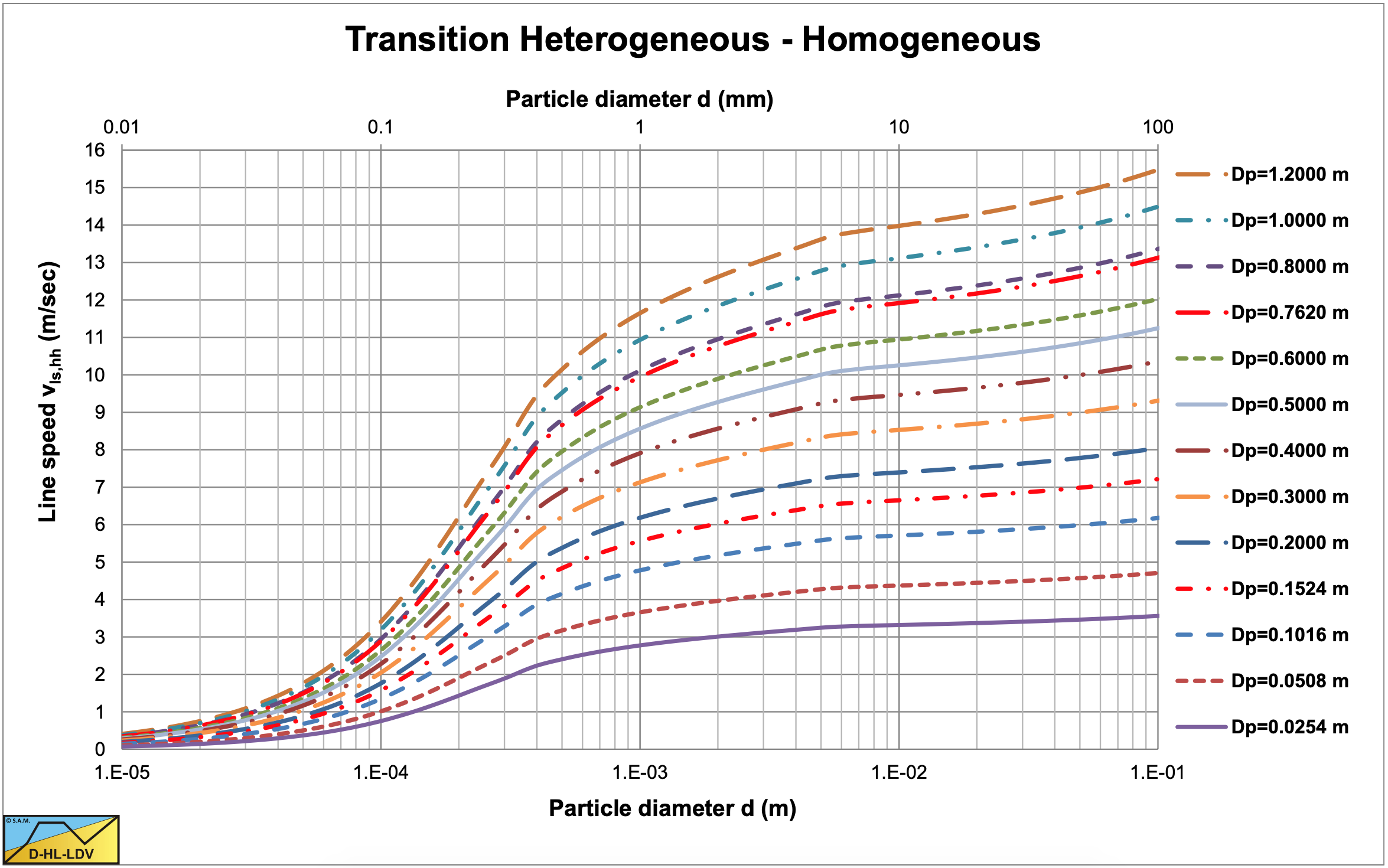
Figure 9.2-1 shows the transition line speed of the Miedema & Ramsdell (2013) DHLLDV Framework as a function of the particle diameter and the pipe diameter.

9.2.3 Durand & Condolios (1952) & Gibert (1960)

The equation for heterogeneous transport of Durand & Condolios (1952) and later Gibert (1960) is:

\[\ \Delta \mathrm{p}_{\mathrm{m}}=\Delta \mathrm{p}_{\mathrm{l}} \cdot\left(\mathrm{1}+\mathrm{\Phi} \cdot \mathrm{C}_{\mathrm{v t}}\right) \quad\text{ or }\quad \mathrm{i}_{\mathrm{m}}=\mathrm{i}_{\mathrm{l}} \cdot\left(\mathrm{1}+\mathrm{\Phi} \cdot \mathrm{C}_{\mathrm{v t}}\right)\]

With:

\[\ \begin{array}{left}\Phi=\frac{\mathrm{i}_{\mathrm{m}}-\mathrm{i}_{\mathrm{l}}}{\mathrm{i}_{\mathrm{l}} \cdot \mathrm{C}_{\mathrm{v t}}}=\frac{\Delta \mathrm{p}_{\mathrm{m}}-\Delta \mathrm{p}_{\mathrm{l}}}{\Delta \mathrm{p}_{\mathrm{l}} \cdot \mathrm{C}_{\mathrm{v t}}}=\mathrm{K} \cdot \Psi^{-\mathrm{3} / 2}=\mathrm{K} \cdot\left(\frac{\mathrm{v}_{\mathrm{l s}}^{2}}{\mathrm{g} \cdot \mathrm{D}_{\mathrm{p}} \cdot \mathrm{R}_{\mathrm{s} \mathrm{d}}} \cdot \sqrt{\mathrm{C}_{\mathrm{x}}}\right)^{-\mathrm{3} / 2}\\
\mathrm{K} \approx \mathrm{8 5}\end{array}\]

The hydraulic gradient in the homogeneous regime, according to ELM so without corrections, is:

\[\ \mathrm{i}_{\mathrm{m}}=\mathrm{i}_{\mathrm{l}} \cdot\left(\mathrm{1}+\mathrm{R}_{\mathrm{s d}} \cdot \mathrm{C}_{\mathrm{v s}}\right) \Rightarrow \frac{\mathrm{i}_{\mathrm{m}}-\mathrm{i}_{\mathrm{l}}}{\mathrm{i}_{\mathrm{l}} \cdot \mathrm{C}_{\mathrm{v s}}}=\frac{\Delta \mathrm{p}_{\mathrm{m}}-\Delta \mathrm{p}_{\mathrm{l}}}{\Delta \mathrm{p}_{\mathrm{l}} \cdot \mathrm{C}_{\mathrm{v s}}}=\mathrm{R}_{\mathrm{s d}}\]

Rewriting this equation into a form that shows the line speed where the heterogeneous transport equation and the homogeneous transport equation are equal, with C_vs=C_vt, gives:

\[\ \mathrm{K} \cdot\left(\frac{\mathrm{v}_{\mathrm{l s}}^{2}}{\mathrm{g} \cdot \mathrm{D}_{\mathrm{p}} \cdot \mathrm{R}_{\mathrm{s} d}} \cdot \sqrt{\mathrm{C}_{\mathrm{x}}}\right)^{-3 / 2}=\frac{\mathrm{1}}{\mathrm{v}_{\mathrm{l} s}^{3}} \cdot \mathrm{K} \cdot\left(\frac{\mathrm{1}}{\mathrm{g} \cdot \mathrm{D}_{\mathrm{p}} \cdot \mathrm{R}_{\mathrm{s} d}} \cdot \sqrt{\mathrm{C}_{\mathrm{x}}}\right)^{-3 / 2}=\mathrm{R}_{\mathrm{s} \mathrm{d}}\]

This gives for the transition velocity between the heterogeneous regime and the homogeneous regime:

\[\ \mathrm{v}_{\mathrm{l s}, \mathrm{h h}}^{\mathrm{3}}=\frac{\mathrm{K}}{\mathrm{R}_{\mathrm{s} \mathrm{d}}} \cdot\left(\frac{\mathrm{g} \cdot \mathrm{D}_{\mathrm{p}} \cdot \mathrm{R}_{\mathrm{s d}}}{\sqrt{\mathrm{C}_{\mathrm{x}}}}\right)^{\mathrm{3 / 2}}\]

This is an explicit equation, which can be solved directly. The Wasp et al. (1977) related models also follow this equation.

9.2.4 Newitt et al. (1955)

The equation for heterogeneous transport of Newitt et al. (1955) is:

\[\ \begin{array}{left} \frac{\mathrm{i}_{\mathrm{m}}-\mathrm{i}_{\mathrm{l}}}{\mathrm{i}_{\mathrm{l}} \cdot \mathrm{C}_{\mathrm{v t}}}=\frac{\Delta \mathrm{p}_{\mathrm{m}}-\Delta \mathrm{p}_{\mathrm{l}}}{\Delta \mathrm{p}_{\mathrm{l}} \cdot \mathrm{C}_{\mathrm{v t}}}=\mathrm{K}_{1} \cdot\left(\mathrm{g} \cdot \mathrm{D}_{\mathrm{p}} \cdot \mathrm{R}_{\mathrm{s} \mathrm{d}}\right) \cdot \mathrm{v}_{\mathrm{t}} \cdot\left(\frac{\mathrm{1}}{\mathrm{v}_{\mathrm{ls}}}\right)^{\mathrm{3}}\\
\mathrm{K}_{1}=\mathrm{1 1 0 0}\end{array}\]

The hydraulic gradient in the homogeneous regime, according to ELM so without corrections, is:

\[\ \mathrm{i}_{\mathrm{m}}=\mathrm{i}_{\mathrm{l}} \cdot\left(\mathrm{1}+\mathrm{R}_{\mathrm{s d}} \cdot \mathrm{C}_{\mathrm{v s}}\right) \Rightarrow \frac{\mathrm{i}_{\mathrm{m}}-\mathrm{i}_{\mathrm{l}}}{\mathrm{i}_{\mathrm{l}} \cdot \mathrm{C}_{\mathrm{v s}}}=\frac{\Delta \mathrm{p}_{\mathrm{m}}-\Delta \mathrm{p}_{\mathrm{l}}}{\Delta \mathrm{p}_{\mathrm{l}} \cdot \mathrm{C}_{\mathrm{v s}}}=\mathrm{R}_{\mathrm{s d}}\]

Rewriting this equation into a form that shows the line speed where the heterogeneous transport equation and the homogeneous transport equation are equal, with C_vs=C_vt, gives:

\[\ \mathrm{K}_{1} \cdot\left(\mathrm{g} \cdot \mathrm{D}_{\mathrm{p}} \cdot \mathrm{R}_{\mathrm{s} \mathrm{d}}\right) \cdot \mathrm{v}_{\mathrm{t}} \cdot\left(\frac{\mathrm{1}}{\mathrm{v}_{\mathrm{l} \mathrm{s}}}\right)^{\mathrm{3}}=\mathrm{R}_{\mathrm{s d}}\]

This gives for the transition velocity between the heterogeneous regime and the homogeneous regime:

\[\ \mathrm{v}_{\mathrm{l} \mathrm{s}, \mathrm{h h}}^{\mathrm{3}}=\mathrm{K}_{\mathrm{1}} \cdot\left(\mathrm{g} \cdot \mathrm{D}_{\mathrm{p}}\right) \cdot \mathrm{v}_{\mathrm{t}}\]

This is an explicit equation, which can be solved directly.

9.2.5 Fuhrboter (1961)

The equation for heterogeneous transport of Fuhrboter (1961) is, using an approximation for the S_k value:

\[\ \begin{array}{left}\mathrm{i}_{\mathrm{m}}=\mathrm{i}_{\mathrm{l}}+\frac{\mathrm{S}_{\mathrm{k}}}{\mathrm{v}_{\mathrm{l s}}} \cdot \mathrm{C}_{\mathrm{v t}} \quad\text{ with: }\quad \mathrm{C}_{\mathrm{v t}}=\mathrm{C}_{\mathrm{v s}}\\
\frac{\mathrm{i}_{\mathrm{m}}-\mathrm{i}_{\mathrm{l}}}{\mathrm{i}_{\mathrm{l}} \cdot \mathrm{C}_{\mathrm{v} \mathrm{s}}}=\frac{\Delta \mathrm{p}_{\mathrm{m}}-\Delta \mathrm{p}_{\mathrm{l}}}{\Delta \mathrm{p}_{\mathrm{l}} \cdot \mathrm{C}_{\mathrm{v} \mathrm{s}}}=\mathrm{R}_{\mathrm{s} \mathrm{d}} \cdot \frac{\mathrm{2} \cdot \mathrm{g} \cdot \mathrm{D}_{\mathrm{p}}}{\lambda_{\mathrm{l}} \cdot \mathrm{v}_{\mathrm{l} \mathrm{s}}^{\mathrm{2}}} \cdot\left(\frac{4 \mathrm{3} . \mathrm{5} \cdot \mathrm{R}_{\mathrm{s d}} \cdot \sqrt{\mathrm{C}_{\mathrm{x}}}^{-1} \cdot \zeta\left(\mathrm{d}_{\mathrm{m}}\right) \cdot\left(v_{\mathrm{l}} \cdot \mathrm{g}\right)^{1 / 3}}{\mathrm{R}_{\mathrm{s d}} \cdot \mathrm{v}_{\mathrm{l} \mathrm{s}}}\right)\\
\text{With : }\quad \zeta\left(\mathrm{d}_{\mathrm{m}}\right)=\left(1-\mathrm{e}^{-\frac{\mathrm{d_m}}{0.0007}} \right)\cdot \left(1+ 10 \cdot \mathrm{e^{-\frac{d_m}{0.00005}}} \right)\end{array}\]

The hydraulic gradient in the homogeneous regime, according to ELM so without corrections, is:

\[\ \mathrm{i}_{\mathrm{m}}=\mathrm{i}_{\mathrm{l}} \cdot\left(\mathrm{1}+\mathrm{R}_{\mathrm{s} \mathrm{d}} \cdot \mathrm{C}_{\mathrm{v} \mathrm{s}}\right) \Rightarrow \frac{\mathrm{i}_{\mathrm{m}}-\mathrm{i}_{\mathrm{l}}}{\mathrm{i}_{\mathrm{l}} \cdot \mathrm{C}_{\mathrm{v s}}}=\frac{\Delta \mathrm{p}_{\mathrm{m}}-\Delta \mathrm{p}_{\mathrm{l}}}{\Delta \mathrm{p}_{\mathrm{l}} \cdot \mathrm{C}_{\mathrm{v s}}}=\mathrm{R}_{\mathrm{s} \mathrm{d}}\]

Rewriting this equation into a form that shows the line speed where the heterogeneous transport equation and the homogeneous transport equation are equal, gives:

\[\ \mathrm{R_{\mathrm{sd}}} \cdot \frac{2 \cdot \mathrm{g} \cdot \mathrm{D}_{\mathrm{p}}}{\lambda_{\mathrm{l}}} \cdot\left(\frac{43.5 \cdot \mathrm{R}_{\mathrm{sd}} \cdot \sqrt{\mathrm{C}_{\mathrm{x}}}^{-1} \zeta\left(\mathrm{d}_{\mathrm{m}}\right) \cdot\left(v_{1} \cdot \mathrm{g}\right)^{1 / 3}}{\mathrm{R}_{\mathrm{sd}}}\right) \cdot\left(\frac{1}{\mathrm{v}_{\mathrm{ls}}}\right)^{3}=\mathrm{R}_{\mathrm{sd}}\]

This gives for the transition velocity between the heterogeneous regime and the homogeneous regime:

\[\ \mathrm{v}_{\mathrm{l} \mathrm{s}, \mathrm{h h}}^{\mathrm{3}}=\frac{\mathrm{2} \cdot \mathrm{g} \cdot \mathrm{D}_{\mathrm{p}}}{\lambda_{\mathrm{l}} \cdot \mathrm{R}_{\mathrm{s d}}} \cdot\left(\mathrm{4 3 .5} \cdot \sqrt{\mathrm{C}_{\mathrm{x}}}^{-\mathrm{1}} \cdot \mathrm{R}_{\mathrm{s d}} \cdot \zeta\left(\mathrm{d}_{\mathrm{m}}\right) \cdot\left(v_{\mathrm{l}} \cdot \mathrm{g}\right)^{1 / \mathrm{3}}\right)=\frac{\mathrm{2} \cdot \mathrm{g} \cdot \mathrm{D}_{\mathrm{p}}}{\lambda_{\mathrm{l}} \cdot \mathrm{R}_{\mathrm{s d}}} \cdot \mathrm{S}_{\mathrm{k}}\]

This is an explicit equation, which can be solved directly.

9.2.6 Jufin & Lopatin (1966)

The equation for heterogeneous transport of Jufin & Lopatin (1966) is, with added terms to make the dimensions correct:

\[\ \begin{array}{left}\Delta \mathrm{p}_{\mathrm{m}}=\Delta \mathrm{p}_{\mathrm{l}} \cdot\left(\mathrm{1}+\mathrm{2} \cdot\left(\frac{\mathrm{v}_{\mathrm{m i n}}}{\mathrm{v}_{\mathrm{l s}}}\right)^{3}\right) \quad\text{ or }\quad \mathrm{i}_{\mathrm{m}}=\mathrm{i}_{\mathrm{l}} \cdot\left(\mathrm{1}+\mathrm{2} \cdot\left(\frac{\mathrm{v}_{\mathrm{m i n}}}{\mathrm{v}_{\mathrm{l s}}}\right)^{3}\right)\\
\mathrm{v}_{\min }=\mathrm{5 .5} \cdot\left(\mathrm{C}_{\mathrm{v t}} \cdot \Psi^{*} \cdot \mathrm{D}_{\mathrm{p}}\right)^{1 / 6} \quad\text{ with: }\quad \Psi^{*}=\left(\frac{\mathrm{v}_{\mathrm{t}}}{\sqrt{\mathrm{g} \cdot \mathrm{d}}}\right)^{3 / 2}\\
\frac{\mathrm{i}_{\mathrm{m}}-\mathrm{i}_{\mathrm{l}}}{\mathrm{i}_{\mathrm{l}} \cdot \mathrm{C}_{\mathrm{v t}}}=2 \cdot \frac{\left(\mathrm{5 . 5} \cdot\left(\mathrm{C}_{\mathrm{v} \mathrm{t}} \cdot\left(\frac{\mathrm{v}_{\mathrm{t}}}{\sqrt{\mathrm{g} \cdot \mathrm{d}}}\right)^{3 / 2} \cdot \mathrm{D}_{\mathrm{p}}\right)^{1 / 6} \cdot \mathrm{7 . 9 2} \cdot\left(\mathrm{g} \cdot \mathrm{R}_{\mathrm{s d}}\right)^{1 / 6} \cdot\left(v_{\mathrm{l}} \cdot \mathrm{g}\right)^{2 / 9}\right)}{\mathrm{C}_{\mathrm{v} \mathrm{t}}} \cdot\left(\frac{\mathrm{1}}{\mathrm{v}_{\mathrm{l} \mathrm{s}}}\right)^{\mathrm{3}}\end{array}\]

The hydraulic gradient in the homogeneous regime, according to ELM so without corrections, is:

\[\ \mathrm{i}_{\mathrm{m}}=\mathrm{i}_{\mathrm{l}} \cdot\left(\mathrm{1}+\mathrm{R}_{\mathrm{s d}} \cdot \mathrm{C}_{\mathrm{v s}}\right) \Rightarrow \frac{\mathrm{i}_{\mathrm{m}}-\mathrm{i}_{\mathrm{l}}}{\mathrm{i}_{\mathrm{l}} \cdot \mathrm{C}_{\mathrm{v s}}}=\frac{\Delta \mathrm{p}_{\mathrm{m}}-\Delta \mathrm{p}_{\mathrm{l}}}{\Delta \mathrm{p}_{\mathrm{l}} \cdot \mathrm{C}_{\mathrm{v s}}}=\mathrm{R}_{\mathrm{s d}}\]

Rewriting this equation into a form that shows the line speed where the heterogeneous transport equation and the homogeneous transport equation are equal, gives:

\[\ 2 \cdot 82654 \cdot\left(\frac{\mathrm{v_{t}}}{\sqrt{\mathrm{g \cdot d}}}\right)^{3 / 4} \cdot\left(\mathrm{g \cdot D_{p} \cdot R_{s d}}\right)^{1 / 2} \cdot\left(v_{\mathrm{l}} \cdot \mathrm{g}\right)^{2 / 3} \cdot\left(\mathrm{C_{v t}}\right)^{-1 / 2}\left(\frac{1}{\mathrm{v_{l s}}}\right)^{3}=\mathrm{R_{s d}}\]

This gives for the transition velocity between the heterogeneous regime and the homogeneous regime:

\[\ \mathrm{v}_{\mathrm{l} \mathrm{s}, \mathrm{h h}}^{\mathrm{3}}=\mathrm{2} \cdot \mathrm{8 2 6 5 4} \cdot\left(\frac{\mathrm{v}_{\mathrm{t}}}{\sqrt{\mathrm{g} \cdot \mathrm{d}}}\right)^{\mathrm{3 / 4}} \cdot\left(\frac{\mathrm{g} \cdot \mathrm{D}_{\mathrm{p}}}{\mathrm{R}_{\mathrm{s d}}}\right)^{1 / 2} \cdot\left(v_{\mathrm{l}} \cdot \mathrm{g}\right)^{2 / 3} \cdot\left(\mathrm{C}_{\mathrm{v t}}\right)^{-1 / 2}\]

This is an explicit equation, which can be solved directly.

9.2.7 Zandi & Govatos (1967)

The final equation for heterogeneous transport of Zandi & Govatos (1967) is:

\[\ \Delta \mathrm{p}_{\mathrm{m}}=\Delta \mathrm{p}_{\mathrm{l}} \cdot\left(\mathrm{1}+\mathrm{2} \mathrm{8} \mathrm{0} \cdot \Psi^{-\mathrm{1} .93} \cdot \mathrm{C}_{\mathrm{v t}}\right)\]

\[\ \Psi=\left(\frac{\mathrm{v}_{\mathrm{l s}}^{2}}{\mathrm{g} \cdot \mathrm{D}_{\mathrm{p}} \cdot \mathrm{R}_{\mathrm{s d}}}\right) \cdot \sqrt{\mathrm{C}_{\mathrm{x}}}\]

The hydraulic gradient in the homogeneous regime, according to ELM so without corrections, is:

\[\ \mathrm{i}_{\mathrm{m}}=\mathrm{i}_{\mathrm{l}} \cdot\left(\mathrm{1}+\mathrm{R}_{\mathrm{s d}} \cdot \mathrm{C}_{\mathrm{v s}}\right) \Rightarrow \frac{\mathrm{i}_{\mathrm{m}}-\mathrm{i}_{\mathrm{l}}}{\mathrm{i}_{\mathrm{l}} \cdot \mathrm{C}_{\mathrm{v s}}}=\frac{\Delta \mathrm{p}_{\mathrm{m}}-\Delta \mathrm{p}_{\mathrm{l}}}{\Delta \mathrm{p}_{\mathrm{l}} \cdot \mathrm{C}_{\mathrm{v s}}}=\mathrm{R}_{\mathrm{s d}}\]

Rewriting this equation into a form that shows the line speed where the heterogeneous transport equation and the homogeneous transport equation are equal, gives:

\[\ 280 \cdot\left(\left(\frac{\mathrm{v}_{\mathrm{ls}}^{2}}{\mathrm{g} \cdot \mathrm{D}_{\mathrm{p}} \cdot \mathrm{R}_{\mathrm{sd}}}\right) \cdot \sqrt{\mathrm{C}_{\mathrm{x}}}\right)^{-1.93}=280 \cdot\left(\frac{\mathrm{g} \cdot \mathrm{D}_{\mathrm{p}} \cdot \mathrm{R}_{\mathrm{sd}}}{\sqrt{\mathrm{C}_{\mathrm{x}}}}\right)^{1.93} \cdot\left(\frac{1}{\mathrm{v}_{\mathrm{ls}}}\right)^{3.86}=\mathrm{R}_{\mathrm{sd}}\]

This gives for the transition velocity between the heterogeneous regime and the homogeneous regime:

\[\ \mathrm{v}_{\mathrm{l} \mathrm{s}, \mathrm{h} \mathrm{h}}^{\mathrm{3.86} }=\mathrm{2} \mathrm{8} \mathrm{0} \cdot\left(\frac{\mathrm{g} \cdot \mathrm{D}_{\mathrm{p}} \cdot \mathrm{R}_{\mathrm{s} \mathrm{d}}}{\sqrt{\mathrm{C}_{\mathrm{x}}}}\right)^{1.93} \cdot \frac{\mathrm{1}}{\mathrm{R}_{\mathrm{s d}}}\]

This is an explicit equation, which can be solved directly.

9.2.8 Turian & Yuan (1977) 1: Saltation Regime

According to Turian & Yuan (1977), the pressure losses with saltating transport can be described by:

\[\ \mathrm{f_{m}-f_{l}=\frac{\lambda_{m}}{4}-\frac{\lambda_{l}}{4}=107.1 \cdot C_{v t}^{1.018} \cdot\left(\frac{\lambda_{l}}{4}\right)^{1.046} \cdot C_{D}^{*-0.4213} \cdot F r^{-1.354}=R_{s d} \cdot C_{v t} \cdot \frac{\lambda_{l}}{4}}\]

This equation can be made equal to the equation for homogeneous transport giving:

\[\ \mathrm{Fr}^{1.354}=107.1 \cdot \mathrm{C}_{\mathrm{vt}}^{1.018} \cdot\left(\frac{\lambda_{\mathrm{l}}}{4}\right)^{0.046} \cdot \mathrm{C}_{\mathrm{D}}^{*-0.4213} \cdot\left(\mathrm{R}_{\mathrm{sd}} \cdot \mathrm{C}_{\mathrm{vt}}\right)^{-1}\]

Rewriting this equation into a form that shows the line speed where the saltating transport equation and the homogeneous transport equation are equal, gives:

\[\ \mathrm{v}_{\mathrm{l s}, \mathrm{h h}}=\left(\mathrm{g} \cdot \mathrm{R}_{\mathrm{s d}} \cdot \mathrm{D}_{\mathrm{p}}\left(\mathrm{1 0 7 . 1} \cdot \mathrm{C _ { v t }}^{\mathrm{1 . 0 1 8}} \cdot\left(\frac{\lambda_{\mathrm{l}}}{\mathrm{4}}\right)^{\mathrm{0 . 0 4 6}} \cdot \mathrm{C}_{\mathrm{D}}^{*-\mathrm{0 . 4 2 1 3}} \cdot\left(\mathrm{R}_{\mathrm{s d}} \cdot \mathrm{C}_{\mathrm{v t}}\right)^{-\mathrm{1}}\right)^{1 / \mathrm{1 . 3 5 4}}\right)^{\mathrm{0 . 5}}\]

The equation of Turian & Yuan (1977) for homogeneous transport is not used here, because we want to compare the intersection point of saltating and homogeneous transport, using the same equation for homogeneous transport for all models.

9.2.9 Turian & Yuan (1977) 2: Heterogeneous Regime

According to Turian & Yuan (1977), the pressure losses with heterogeneous transport can be described by:

\[\ \mathrm{f_{m}-f_{l}=\frac{\lambda_{m}}{4}-\frac{\lambda_{l}}{4}=30.11 \cdot C_{v t}^{0.868} \cdot\left(\frac{\lambda_{l}}{4}\right)^{1.200} \cdot C_{D}^{*-0.1677} \cdot F r^{-0.6938}=R_{s d} \cdot C_{v t} \cdot \frac{\lambda_{l}}{4}}\]

This equation can be made equal to the equation for homogeneous transport giving:

\[\ \operatorname{Fr}^{0.6938}=30.11 \cdot \mathrm{C}_{\mathrm{vt}}^{0.868} \cdot\left(\frac{\lambda_{\mathrm{l}}}{4}\right)^{0.200} \cdot \mathrm{C}_{\mathrm{D}}^{*-0.1677} \cdot\left(\mathrm{R}_{\mathrm{sd}} \cdot \mathrm{C}_{\mathrm{vt}}\right)^{-1}\]

Rewriting this equation into a form that shows the line speed where the heterogeneous transport equation and the homogeneous transport equation are equal, gives:

\[\ \mathrm{v}_{\mathrm{l s}, \mathrm{h h}}=\left(\mathrm{g} \cdot \mathrm{R}_{\mathrm{s d}} \cdot \mathrm{D}_{\mathrm{p}}\left(\mathrm{3 0 . 1 1} \cdot \mathrm{C}_{\mathrm{v t}}^{\mathrm{0 . 8 6 8}} \cdot\left(\frac{\lambda_{\mathrm{l}}}{\mathrm{4}}\right)^{0 . \mathrm{2 0 0}} \cdot \mathrm{C}_{\mathrm{D}}^{*-\mathrm{0 . 1 6 7 7}} \cdot\left(\mathrm{R}_{\mathrm{s d}} \cdot \mathrm{C}_{\mathrm{v t}}\right)^{-1}\right)^{1 / 0.6938}\right)^{0.5}\]

The equation of Turian & Yuan (1977) for homogeneous transport is not used here, because we want to compare the intersection point of heterogeneous and homogeneous transport, using the same equation for homogeneous transport for all models.

9.2.10 Wilson et al. (1992) (Power 1.0, Non-Uniform Particles)

The final simplified equation for heterogeneous transport of Wilson et al. (1992) is:

\[\ \frac{\mathrm{i}_{\mathrm{m}}-\mathrm{i}_{\mathrm{l}}}{\mathrm{i}_{\mathrm{l}} \cdot \mathrm{C}_{\mathrm{v t}}}=\frac{\Delta \mathrm{p}_{\mathrm{m}}-\Delta \mathrm{p}_{\mathrm{l}}}{\Delta \mathrm{p}_{\mathrm{l}} \cdot \mathrm{C}_{\mathrm{v s}}}=\mathrm{4 4 . 1} ^{\mathrm{M}} \cdot \frac{\mu_{\mathrm{s f}} \cdot \mathrm{g} \cdot \mathrm{R}_{\mathrm{s d}} \cdot \mathrm{D}_{\mathrm{p}}}{\lambda_{\mathrm{l}}} \cdot\left(\mathrm{d}_{\mathrm{5 0}}\right)^{\mathrm{0 . 3 5} \cdot \mathrm{M}} \cdot\left(\frac{\mathrm{1}}{\mathrm{v}_{\mathrm{l s}}}\right)^{\mathrm{2}+\mathrm{M}}\]

The hydraulic gradient in the homogeneous regime, according to ELM so without corrections, is:

\[\ \mathrm{i}_{\mathrm{m}}=\mathrm{i}_{\mathrm{l}} \cdot\left(\mathrm{1}+\mathrm{R}_{\mathrm{s d}} \cdot \mathrm{C}_{\mathrm{v s}}\right) \Rightarrow \frac{\mathrm{i}_{\mathrm{m}}-\mathrm{i}_{\mathrm{l}}}{\mathrm{i}_{\mathrm{l}} \cdot \mathrm{C}_{\mathrm{v s}}}=\frac{\Delta \mathrm{p}_{\mathrm{m}}-\Delta \mathrm{p}_{\mathrm{l}}}{\Delta \mathrm{p}_{\mathrm{l}} \cdot \mathrm{C}_{\mathrm{v s}}}=\mathrm{R}_{\mathrm{s d}}\]

Rewriting this equation into a form that shows the line speed where the heterogeneous transport equation and the homogeneous transport equation are equal, gives:

\[\ 44.1^{\mathrm{M}} \cdot \frac{\mu_{\mathrm{sf}} \cdot \mathrm{g} \cdot \mathrm{R}_{\mathrm{sd}} \cdot \mathrm{D}_{\mathrm{p}}}{\lambda_{\mathrm{l}}} \cdot\left(\mathrm{d}_{50}\right)^{0.35 \cdot \mathrm{M}} \cdot\left(\frac{1}{\mathrm{v}_{\mathrm{ls}}}\right)^{2+\mathrm{M}}=\mathrm{R}_{\mathrm{sd}}\]

This gives for the transition velocity between the heterogeneous regime and the homogeneous regime for M=1:

\[\ \mathrm{v}_{\mathrm{l} \mathrm{s}, \mathrm{h h}}^{\mathrm{3}}=\mathrm{4 4 .1} \cdot \frac{\boldsymbol{\mu}_{\mathrm{s f}} \cdot \mathrm{g} \cdot \mathrm{D}_{\mathrm{p}}}{\lambda_{\mathrm{l}}} \cdot\left(\mathrm{d}_{\mathrm{5} 0}\right)^{0.35}\]

It should be mentioned that this is based on the simplifie model of Wilson et al. (1992) for heterogeneous transport. The full model may give slightly different results.

9.2.11 Wilson et al. (1992) (Power 1.7, Uniform Particles)

The final simplified equation for heterogeneous transport of Wilson et al. (1992) is:

\[\ \frac{\mathrm{i}_{\mathrm{m}}-\mathrm{i}_{\mathrm{l}}}{\mathrm{i}_{\mathrm{l}} \cdot \mathrm{C}_{\mathrm{v t}}}=\frac{\Delta \mathrm{p}_{\mathrm{m}}-\Delta \mathrm{p}_{\mathrm{l}}}{\Delta \mathrm{p}_{\mathrm{l}} \cdot \mathrm{C}_{\mathrm{v s}}}=44.1^{\mathrm{M}} \cdot \frac{\mu_{\mathrm{s f}} \cdot \mathrm{g} \cdot \mathrm{R}_{\mathrm{s d}} \cdot \mathrm{D}_{\mathrm{p}}}{\lambda_{\mathrm{l}}} \cdot\left(\mathrm{d}_{\mathrm{5 0}}\right)^{\mathrm{0 . 3 5} \cdot \mathrm{M}} \cdot\left(\frac{\mathrm{1}}{\mathrm{v}_{\mathrm{l s}}}\right)^{\mathrm{2 + M}}\]

The hydraulic gradient in the homogeneous regime, according to ELM so without corrections, is:

\[\ \mathrm{i}_{\mathrm{m}}=\mathrm{i}_{\mathrm{l}} \cdot\left(\mathrm{1}+\mathrm{R}_{\mathrm{s d}} \cdot \mathrm{C}_{\mathrm{v s}}\right) \Rightarrow \frac{\mathrm{i}_{\mathrm{m}}-\mathrm{i}_{\mathrm{l}}}{\mathrm{i}_{\mathrm{l}} \cdot \mathrm{C}_{\mathrm{v s}}}=\frac{\Delta \mathrm{p}_{\mathrm{m}}-\Delta \mathrm{p}_{\mathrm{l}}}{\Delta \mathrm{p}_{\mathrm{l}} \cdot \mathrm{C}_{\mathrm{v s}}}=\mathrm{R}_{\mathrm{s d}}\]

Rewriting this equation into a form that shows the line speed where the heterogeneous transport equation and the homogeneous transport equation are equal, gives:

\[\ 44.1^{\mathrm{M}} \cdot \frac{\mu_{\mathrm{sf}} \cdot \mathrm{g} \cdot \mathrm{R}_{\mathrm{sd}} \cdot \mathrm{D}_{\mathrm{p}}}{\lambda_{\mathrm{l}}} \cdot\left(\mathrm{d}_{50}\right)^{0.35 \cdot \mathrm{M}} \cdot\left(\frac{1}{\mathrm{v}_{\mathrm{ls}}}\right)^{2+\mathrm{M}}=\mathrm{R}_{\mathrm{sd}}\]

This gives for the transition velocity between the heterogeneous regime and the homogeneous regime:

\[\ \mathrm{v}_{\mathrm{l} \mathrm{s}, \mathrm{h h}}^{\mathrm{3 .7}}=\mathrm{4 4 .1}^{\mathrm{1 . 7}} \cdot \frac{\boldsymbol{\mu}_{\mathrm{s f}} \cdot \mathrm{g} \cdot \mathrm{D}_{\mathrm{p}}}{\lambda_{\mathrm{l}}} \cdot\left(\mathrm{d}_{\mathrm{5 0}}\right)^{\mathrm{0 . 3 5} \cdot {1 . 7}}\]

It should be mentioned that this is based on the simplified model of Wilson et al. (1992) for heterogeneous transport. The full model may give slightly different results.

9.2.12 Wilson & Sellgren (2012) Near Wall Lift Model

The relative excess hydraulic gradient of the near wall lift model is:

\[\ \mathrm{E}_{\mathrm{rhg}}=\mathrm{R}=\frac{\mathrm{1 0} \cdot\left(\mathrm{R}_{\mathrm{sd}} \cdot \mathrm{g} \cdot \mathrm{d}\right)^{1 / 2} \cdot\left(\mathrm{R}_{\mathrm{s d}} \cdot \mathrm{g} \cdot v_{\mathrm{l}}\right)^{1 / 3}}{\lambda_{\mathrm{l}} \cdot \mathrm{v}_{\mathrm{l} \mathrm{s}}^{2}}\]

The near wall lift based equation gives for sand and water:

\[\ \mathrm{E}_{\mathrm{rhg}}=\mathrm{R}=\frac{\mathrm{d}^{1 / 2}}{\lambda_{\mathrm{l}} \cdot \mathrm{v}_{\mathrm{ls}}^{2}}\]

The relative excess hydraulic gradient in the homogeneous regime, according to ELM so without corrections, is:

\[\ \mathrm{E}_{\mathrm{r h g}}=\frac{\mathrm{i}_{\mathrm{m}}-\mathrm{i}_{\mathrm{l}}}{\mathrm{R}_{\mathrm{s d}} \cdot \mathrm{C}_{\mathrm{v s}}}=\mathrm{i}_{\mathrm{l}}=\frac{\lambda_{\mathrm{l}} \cdot \mathrm{v}_{\mathrm{l s}}^{\mathrm{2}}}{\mathrm{2} \cdot \mathrm{g} \cdot \mathrm{D}_{\mathrm{p}}}\]

This gives for the transition velocity between the heterogeneous regime and the homogeneous regime:

\[\ \mathrm{v}_{\mathrm{ls}, \mathrm{h h}}^{4}=\frac{\mathrm{2} \cdot \mathrm{g} \cdot \mathrm{D}_{\mathrm{p}}}{\lambda_{\mathrm{l}}^{2}} \cdot \mathrm{d}^{1 / 2}\]

9.2.13 The Saskatchewan Research Council Model

The SRC model consists of two terms regarding the excess hydraulic gradient. A term for the contact load and a term for the suspended load. Here only the term for the contact load is considered, assuming the contact load results in a small bed and there is no buoyancy from the suspended load.

The hydraulic gradients of the heterogeneous (contact load) model should be equal to the homogeneous model giving:

\[\ \mu_{\mathrm{sf}} \cdot \mathrm{e}^{-0.0212 \cdot \frac{\mathrm{v}_{\mathrm{ls}, \mathrm{hh}}}{\mathrm{v}_{\mathrm{t}}}} \cdot \mathrm{R}_{\mathrm{sd}} \cdot \mathrm{C}_{\mathrm{vs}}=\frac{\lambda_{\mathrm{l}} \cdot \mathrm{v}_{\mathrm{ls}, \mathrm{hh}}^{2}}{2 \cdot \mathrm{g} \cdot \mathrm{D}_{\mathrm{p}}} \cdot \mathrm{R}_{\mathrm{sd}} \cdot \mathrm{C}_{\mathrm{vs}}\]

The SRC model results in an implicit relation if only the contact load is considered, this gives:

\[\ \mathrm{v}_{\mathrm{ls}, \mathrm{h} \mathrm{h}}^{2}=\mu_{\mathrm{s f}} \cdot \mathrm{e}^{-\mathrm{0} . \mathrm{0 2 1 2} \cdot \frac{\mathrm{v}_{\mathrm{ls}, \mathrm{hh}}}{\mathrm{v}_{\mathrm{t}}}} \cdot {\frac{\mathrm{2} \cdot \mathrm{g} \cdot \mathrm{D}_{\mathrm{p}}}{\lambda_{\mathrm{l}}}} \quad\text{ or }\quad \mathrm{v}_{\mathrm{l} \mathrm{s}, \mathrm{h h}}^{\mathrm{2}} \cdot \mathrm{e}^{\mathrm{0} \cdot \mathrm{0 2 1 2} \cdot \frac{\mathrm{v}_{\mathrm{ls}, \mathrm{h h}}}{\mathrm{v_{t}}}}=\mu_{\mathrm{s f}} \cdot \frac{\mathrm{2} \cdot \mathrm{g} \cdot \mathrm{D}_{\mathrm{p}}}{\lambda_{\mathrm{l}}}\]

9.2.14 Examples Heterogeneous versus Homogeneous

The comparison is based on models for saltating or heterogeneous transport. As mentioned before, the transition line speed from heterogeneous to homogeneous transport is a good indicator for the excess pressure losses. A higher transition line speed indicates higher excess pressure losses. For a pipe diameter of 0.1016 m (4 inch) and medium sized particles (0.1 mm to 2 mm) all models are close for high concentrations (around 30%), shown in Figure 9.2-10. This is caused by the fact that most experiments are carried out in small diameter pipes, resulting in a cloud of data points because of scatter. Many curves will fit through this cloud of data points.

The following graphs (Figure 9.2-5, Figure 9.2-6, Figure 9.2-7, Figure 9.2-8 Figure 9.2-9, Figure 9.2-10, Figure 9.2-11, Figure 9.2-12, Figure 9.2-13, Figure 9.2-14, Figure 9.2-15, Figure 9.2-16, Figure 9.2-17 and Figure 9.2-18) have a dimensionless vertical axis by dividing the transition line speed by the maximum transition line speed occurring in one of the 11 models. This maximum transition line speed is shown in the lower right corner of each graph. For normal dredging operations, particles diameters from 0.1 mm up to 10 mm are of interests. The different models are compared with the DHLLDV Framework of Miedema & Ramsdell (2013). For very small pipe diameters (<0.1 m) the Newitt et al. (1955) model is representative, for medium pipe diameters (0.1-0.3 m) the Fuhrboter (1961) model and the Durand & Condolios (1952) model are representative and for large pipe diameters (>0.3 m) the Jufin & Lopatin (1966) model is representative, although this model tends to underestimate the pressure losses slightly for large pipe diameters and high concentrations. The Wilson et al. (1992) and the SRC models have developed over the years and are based on many experimental data and can thus be considered to be representative in all cases for medium sized particles.

In the following paragraphs the influence of 6 parameters on the transition velocity between the heterogeneous and the homogeneous regimes is discussed. When the word model is used, it refers to the model or equation of this transition velocity.

9.2.14.1 The Influence of the Particle Diameter & Terminal Settling Velocity

Two groups of models can be distinguished.
The first group: models based on the terminal settling velocity, Newitt et al. (1955) and the SRC model, or a directly related parameter, Wilson et al. (1992). The small DHLLDV Framework potential energy term also depends on the hindered settling velocity.
The second group: models based on the particle Froude number, Durand & Condolios (1952), Jufin & Lopatin (1966) (values from a table) and the large DHLLDV Framework kinetic energy term, or based on the particle drag coefficient, Fuhrboter (1961) (values from a graph), Zandi & Govatos (1967) and Turian & Yuan (1977). The difference between the particle Froude number and the particle drag coefficient is mainly the relative submerged density and a constant. In other words, the particle drag coefficient is independent of the relative submerged density, while the particle Froude number is dependent. As long as sand and gravel are considered, the two are related by a fixed factor, but for other solids this factor changes.

The difference between the two groups is, that the terminal settling velocity continuously increases with the particle diameter, while the particle Froude number and the particle drag coefficient have a constant asymptotic value for large particle diameters.
So models from the first group tend to overestimate the transition line speed for large particles. This is however not surprising, since both Newitt et al. (1955), SRC and Wilson et al. (1992) use a 2LM or sliding bed model for this case, so the large particle part of the curves is not relevant.

9.2.14.2 The Influence of the Pipe Diameter

Some models give a direct relation between the transition velocity and the pipe diameter, other models include the Darcy Weisbach friction factor which decreases with the pipe diameter with a power of about 0.2. For these models the powers mentioned are an estimate.
The Durand & Condolios (1952) and Zandi & Govatos (1967) models show a proportionality of the transition line speed with the pipe diameter with a power of 0.5. The two Turian & Yuan (1977) models also. The Newitt et al. (1955) model shows a proportionality with a power of 1/3. Fuhrboter (1961) also a power of 1/3. Jufin & Lopatin (1966) a power of 1/6. The two Wilson et al. (1992) models 0.3-0.4. The SRC model about 0.2 for small particles (d=0.1 mm), 0.3 for medium particles (d=0.4 mm), 0.4 for medium/coarse particles (d=1 mm) and 0.5 for large particles (d=10 mm), due to the exponential function in the equation. This results in a proportionality power related to the terminal settling velocity. Finally the DHLLDV Framework with a power of about 0.35.

In general one can say that the transition line speed is proportional to the pipe diameter with a power of 0.3 to 0.4, based on the Wilson et al. (1992) models, the SRC model and the DHLLDV Framework.

9.2.14.3 The Influence of the Concentration

The model of Jufin & Lopatin (1966) strongly depends on the volumetric concentration, the DHLLDV Framework of Miedema & Ramsdell (2013) weakly as well as the models of Turian & Yuan (1977). Turian & Yuan (1977) saltating has a small positive power (+0.13), while the heterogeneous equation shows a small negative power (- 0.22). Jufin & Lopatin (1966) give a power of -1/6. These small negative powers match the DHLLDV Framework for homogeneous flow based on a particle free viscous sub-layer. The DHLLDV Framework heterogeneous model consists of a potential energy term and a kinetic energy term. The small potential energy term depends on the concentration due to the hindered settling effect.

The models of Durand & Condolios (1952) & Gibert (1960), Newitt et al. (1955), Fuhrboter (1961), Zandi & Govatos (1967), Wilson et al. (1992) and the SRC model do not depend on the volumetric concentration.
In general one can say that the transition line speed depends weakly on the spatial concentration.

9.2.14.4 The Influence of the Sliding Friction Coefficient

The Wilson et al. (1992) and the SRC models are based on a sliding bed and a stratification ratio. It is assumed that the heterogeneous regime consists of a sliding bed of which the thickness decreases with increasing line speed according to a certain relation. Since the excess head losses of a sliding bed are proportional to the sliding friction factor, so is the transition velocity. The power of this proportionality is between 1/3 and 1/4. However, since the sliding friction coefficient does not vary much, this parameter is not very important. Wilson et al. (1992) uses values of 0.4 and 0.44, while SRC advises 0.5. All other models do not use the sliding friction coefficient.

In general one can say that there is no influence of the sliding friction coefficient on the transition velocity of the heterogeneous and the homogeneous regimes.

9.2.14.5 The Influence of the Relative Submerged Density

In the DHLLDV Framework there is no direct influence of the relative submerged density, only an indirect influence through the particle Froude number. The Durand & Condolios (1952) model shows a weak influence with a power of 1/6 and an indirect influence through the particle Froude number. The Newitt et al. (1955) model is independent of the relative submerged density, for the transition velocity. Apparently the influence of the relative submerged density on the heterogeneous and the homogeneous (ELM) regimes is the same. The Fuhrboter (1961) model gives the same conclusion with the approximation equation for the S_k value. The original Jufin & Lopatin (1966) model only depends indirectly through the particle Froude number on the relative submerged density. The Zandi & Govatos (1967) model depends both directly and indirectly on the relative submerged density. Directly with a power of about 0.25. The Turian & Yuan (1977) models depend weakly on the relative submerged density with powers of +0.15 and -0.2. The Wilson et al. (1992) models and the SRC model do not depend on the relative submerged density.

In general one can say that there is a weak or no direct dependency of the transition velocity of the heterogeneous and the homogeneous regimes on the relative submerged density. Some models give a weak indirect dependency on the particle Froude number.

9.2.14.6 The Influence of the Line Speed

In the models of Durand & Condolios (1952), Newitt et al. (1955), Fuhrboter (1961), Jufin & Lopatin (1966) and Wilson et al. (1992) (the -1 power model) the pressure losses or hydraulic gradient decreases reversely with the line speed.
The Zandi & Govatos (1967), Wilson et al. (1992) (the -1.7 power model) and the DHLLDV Framework with a power between -1.7 and -2.0.

The Turian & Yuan (1977) saltating regime has a power of about -0.7, while the Turian & Yuan (1977) heterogeneous equation has a positive power of about +0.6. These powers are probably the result of curve fitting of experimental data in the sliding bed + the heterogeneous regimes (powers of 0 and -1 to -2), resulting in the power of -0.7 and data in the heterogeneous + the (pseudo) homogeneous regimes (powers of -1 to -2 and +2), resulting in the power of +0.6.

In general one can say that the more negative the power of the line speed in the heterogeneous hydraulic gradient equation, the smaller the transition velocity between the regimes. One has to take this into account interpreting the graphs.

9.2.14.7 Summary

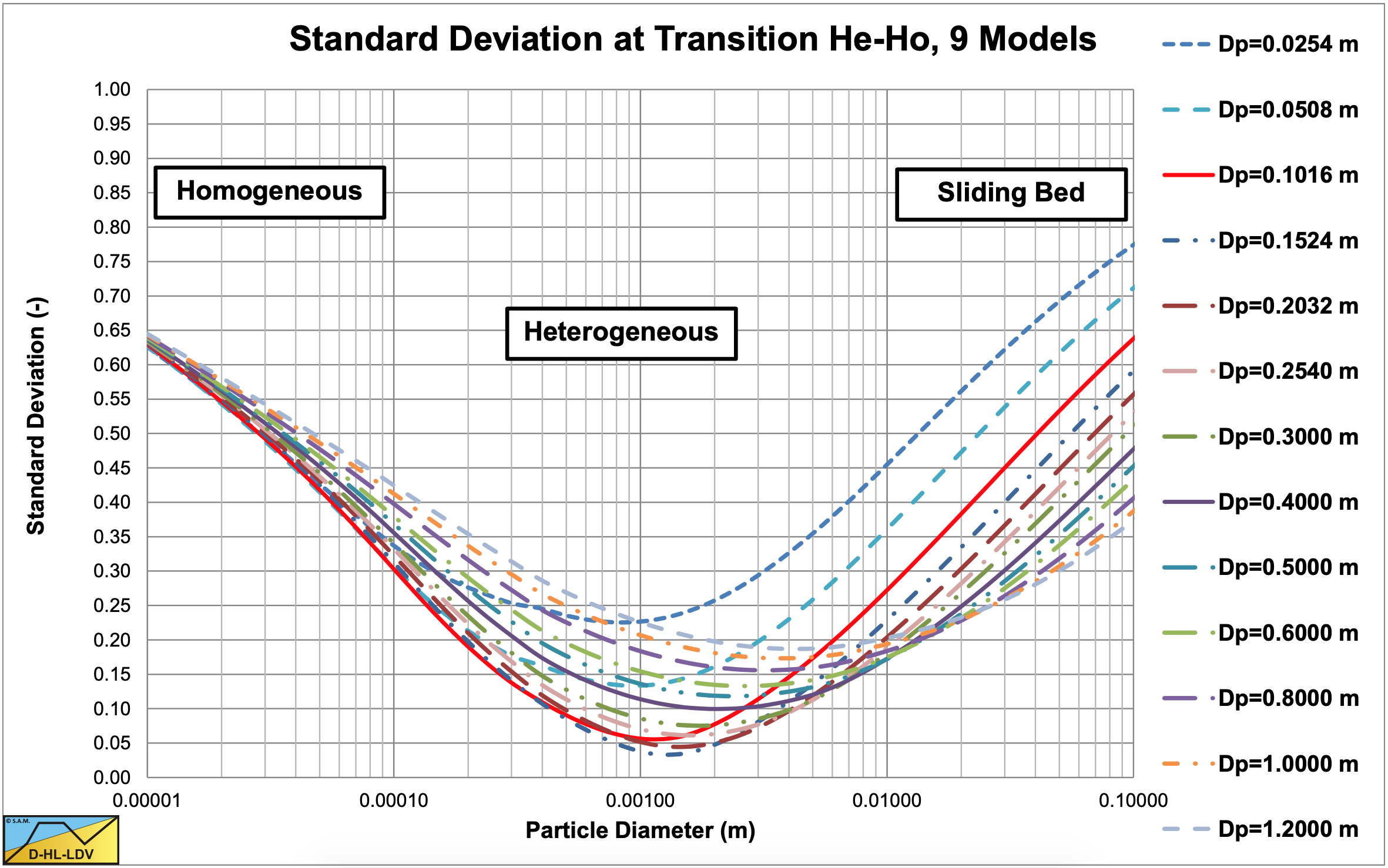
The standard deviation of the 12 models for C_vs=0.175 is shown in Figure 9.2-2. For pipe diameters close to 0.1016 m (4 inch) and particle diameters in the range of 0.3 to 4 mm, the standard deviation is less than 10%. This is also the particle diameter region of heterogeneous transport. Smaller pipes and larger pipes show a larger standard deviation. This means that for pipe diameters close to 0.1016 m and particles in the range of 0.3 to 4 mm, all models give about the same result in terms of the solids effect in the hydraulic gradient. The smaller the pipe or the larger the pipe the more the models deviate. Figure 9.2-3 shows the standard deviation omitting the 3 Wilson et al. models, since these give very high transition velocities for very small particles. The same trends are observed here.

Figure 9.2-2: The standard deviation of 12 models.

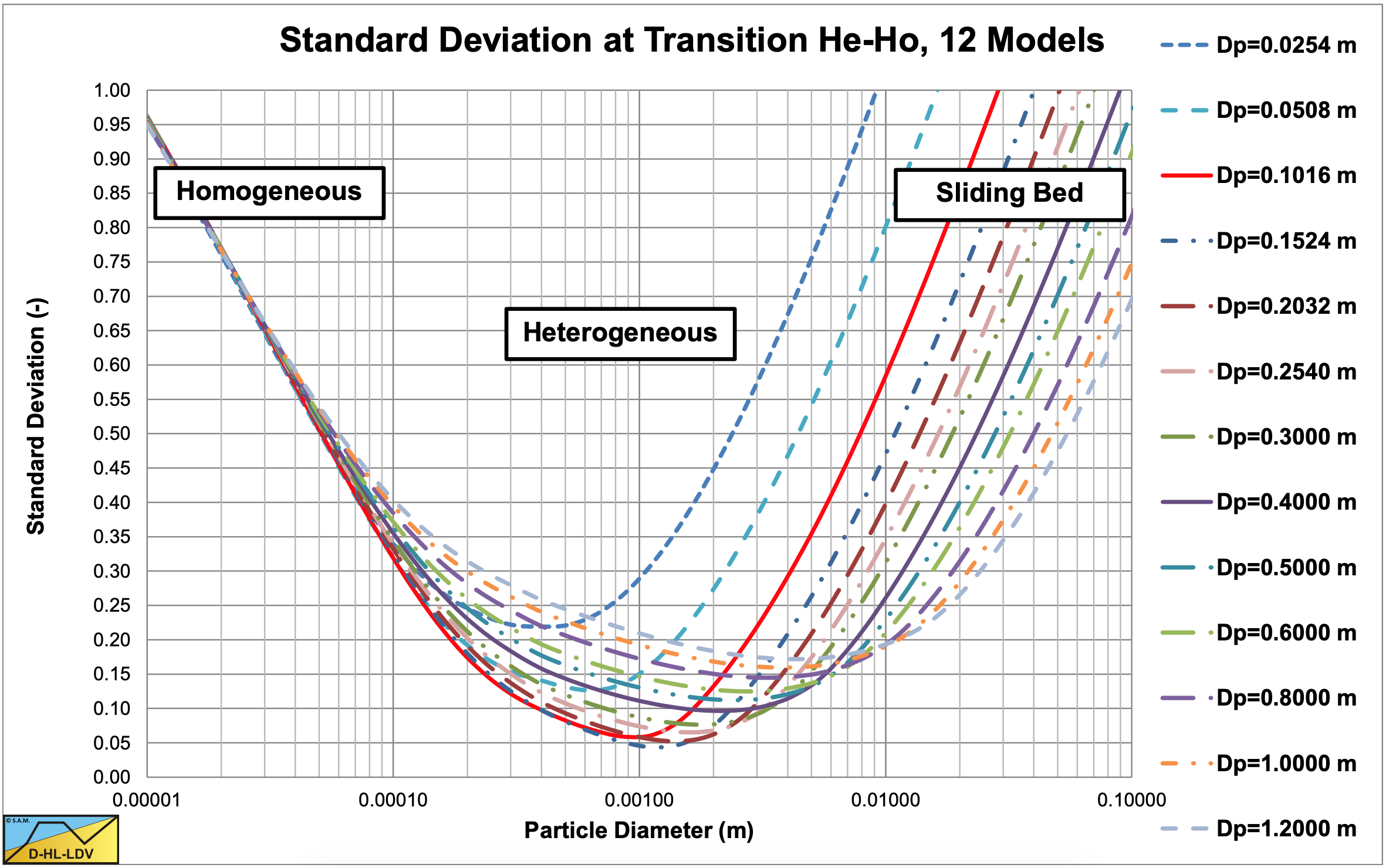
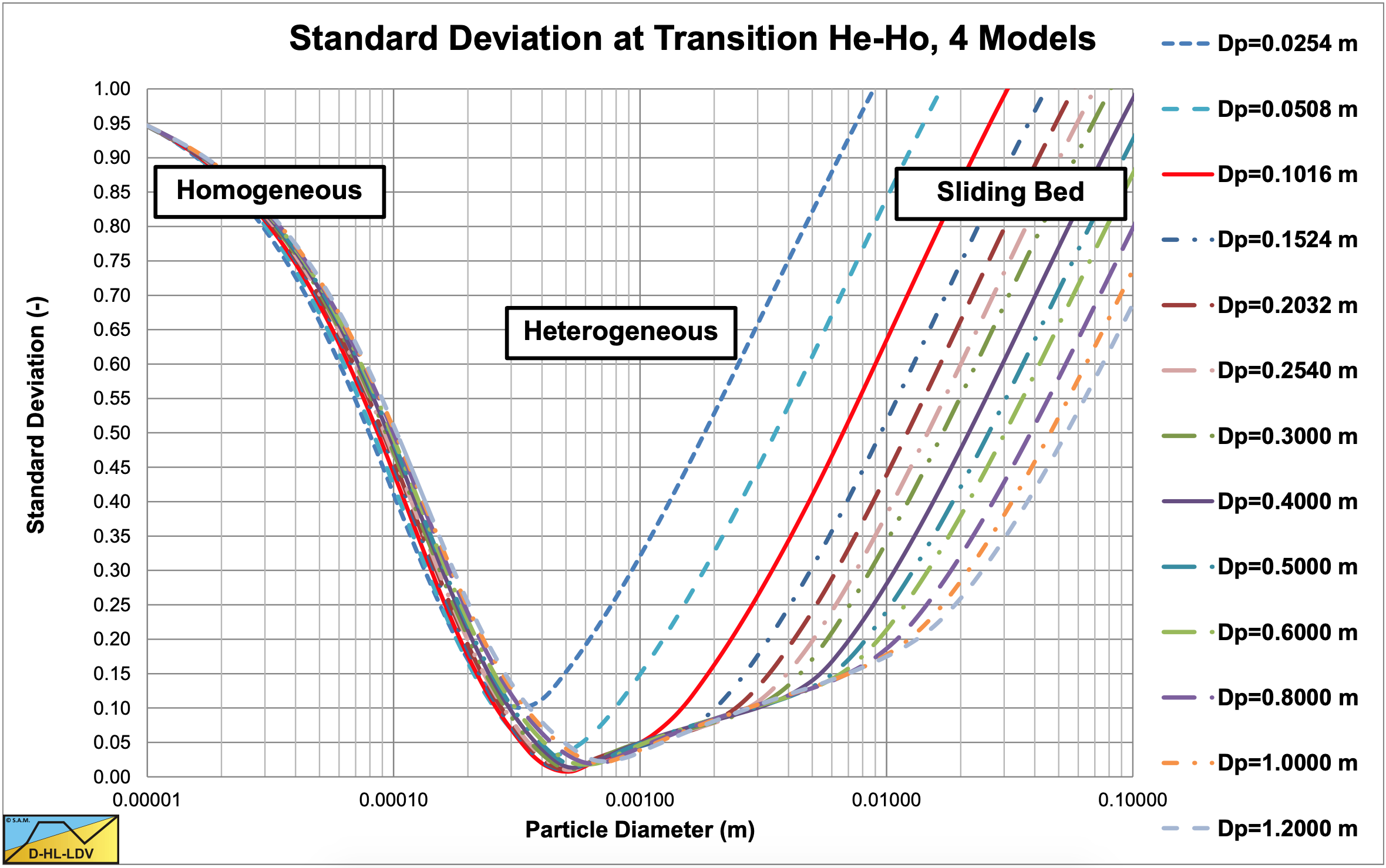
Figure 9.2-4 shows the standard deviation of the DHLLDV Framework, the SRC model and the Wilson et al. models with a power of 1.7 and the near wall lift method (NWL). In the range of particle diameters from 0.25 mm to 1-3 mm the standard deviation is less than 10% and does not really depend on the pipe diameter. Very small particles show a high standard deviation, but the heterogeneous models are not applicable there. At normal operational line speeds, which are much higher than the transition line speeds found, the transport will be according

to the homogeneous flow regime (ELM related). Very large particles show an increasing standard deviation, resulting from the fact that here the sliding bed or sliding flow regimes are applicable and not the heterogeneous flow regime.
Although the physics behind the 4 models considered, the DHLLDV Framework, the SRC model and the 2 Wilson et al. models, are different, the 4 models give about the same result for medium sands in terms of the solids effect, irrespective of the pipe diameter.

Figure 9.2-3: The standard deviation of 9 models.

Figure 9.2-4: The standard deviation of 4 models

9.2.14.8 A 0.0254 m Diameter Pipe (1 inch)

Figure 9.2-5: The transition line speed He-Ho for D_p=0.0254 m and C_v=0.05.

Figure 9.2-6: The transition line speed He-Ho for D_p=0.0254 m and C_v=0.30.

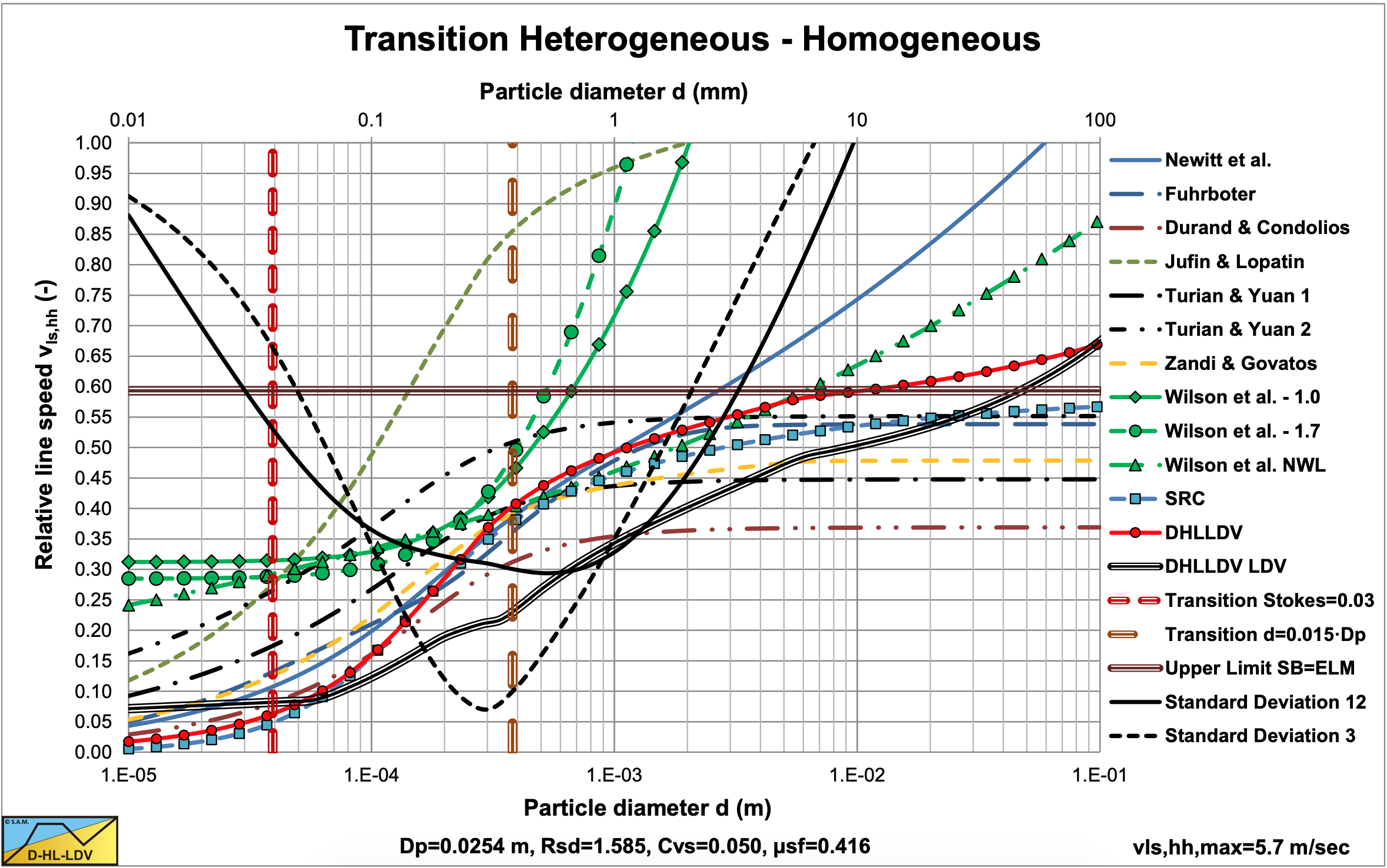
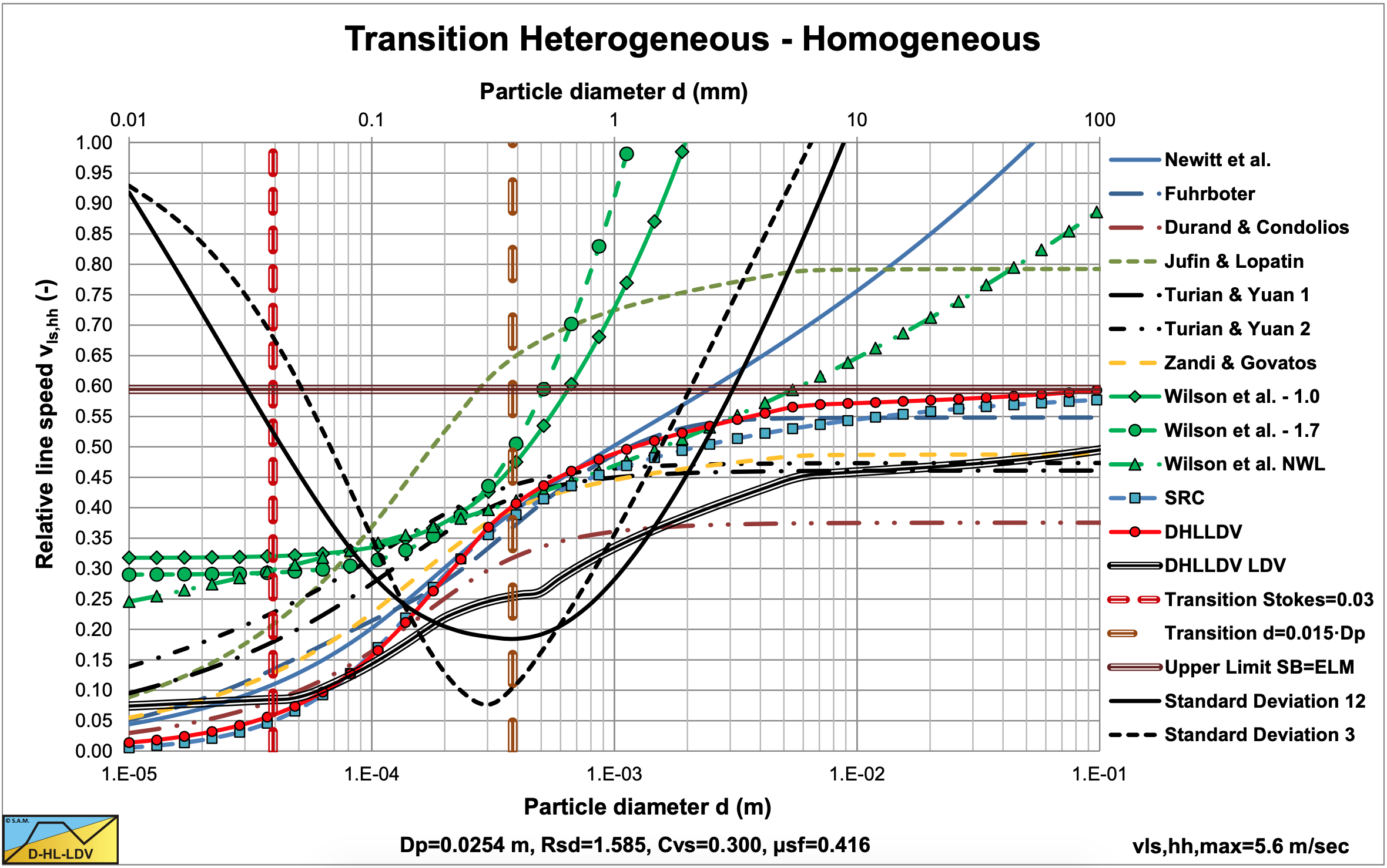
In the range of medium sized particles most models are very close. The Durand & Condolios model however seems to underestimate the transition velocity, while the Jufin & Lopatin and the Turian & Yuan 2 models overestimate the transition velocity. The SRC and the DHLLDV Framework are very close up to a particle size of about 10 mm.

9.2.14.9 A 0.0508 m Diameter Pipe (2 inch)

Figure 9.2-7: The transition line speed He-Ho for D_p=0.0508 m and C_v=0.05

Figure 9.2-8: The transition line speed He-Ho for D_p=0.0508 m and C_v=0.30

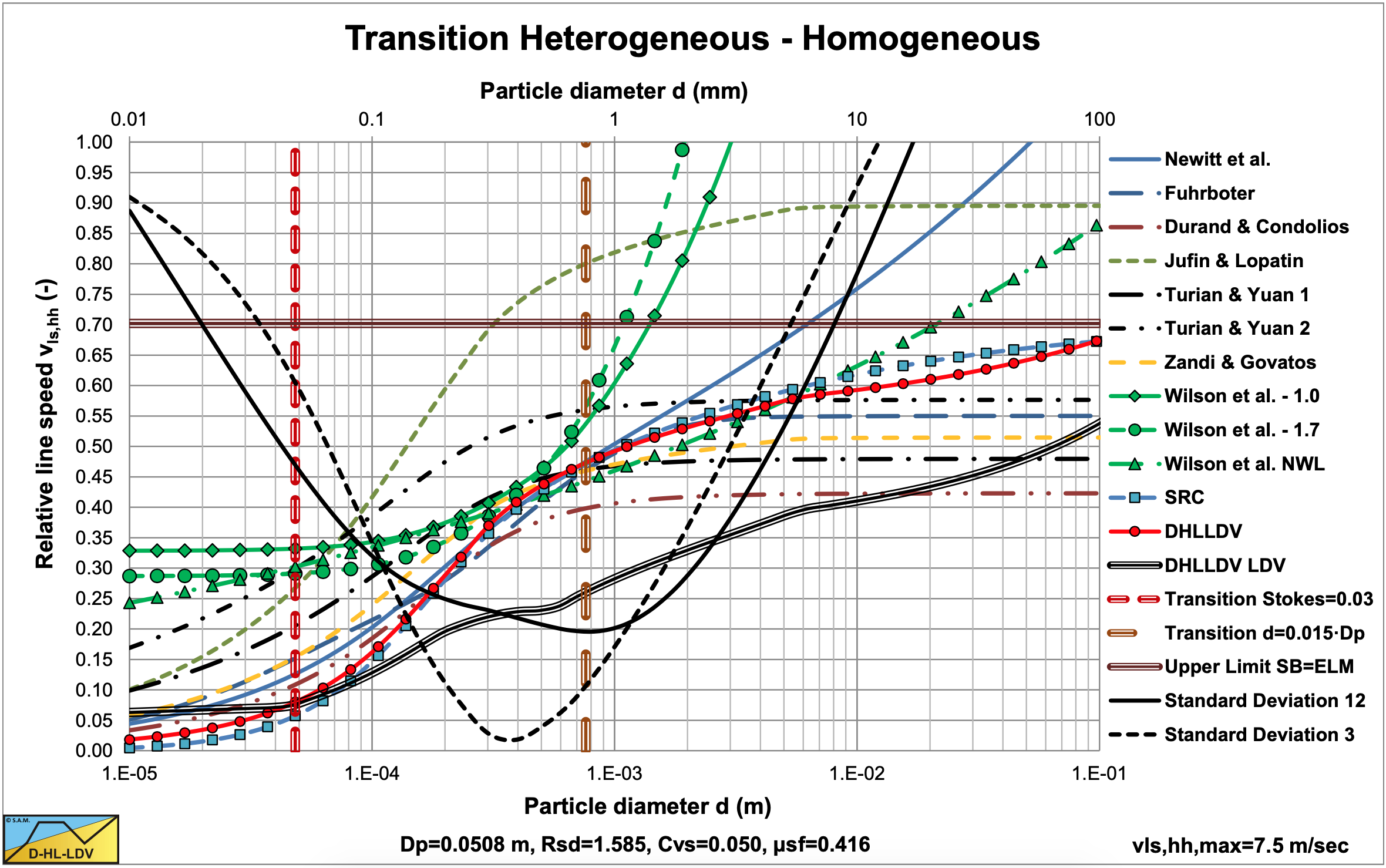
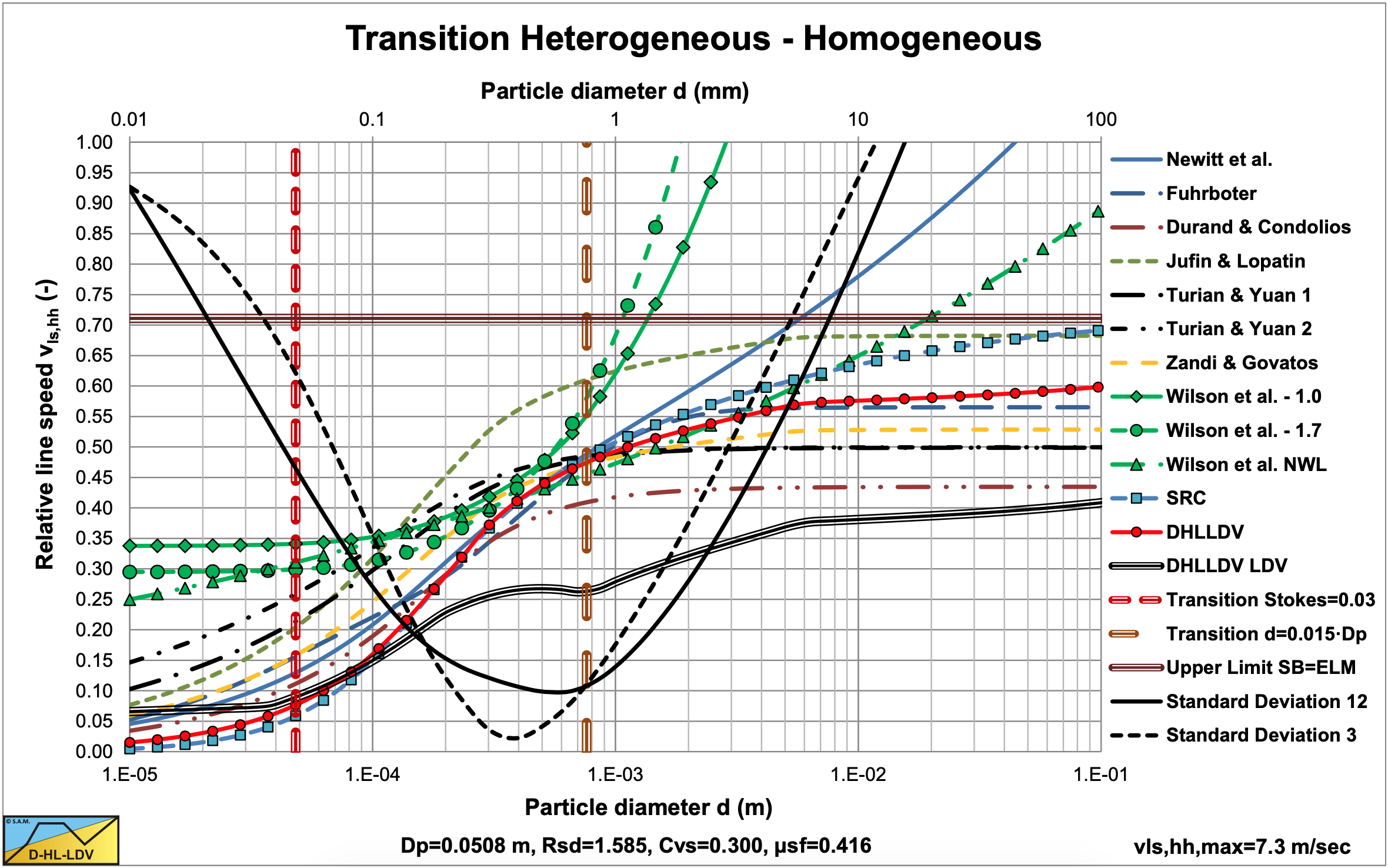
In the range of medium sized particles most models are very close. The Durand & Condolios model however seems to underestimate the transition velocity, while the Jufin & Lopatin and the Turian & Yuan 2 models overestimate the transition velocity. The SRC and the DHLLDV Framework are very close up to a particle size of about 2 mm.

9.2.14.10 A 0.1016 m Diameter Pipe (4 inch)

Figure 9.2-9: The transition line speed He-Ho for D_p=0.1016 m and C_v=0.05

Figure 9.2-10: The transition line speed He-Ho for D_p=0.1016 m and C_v=0.30

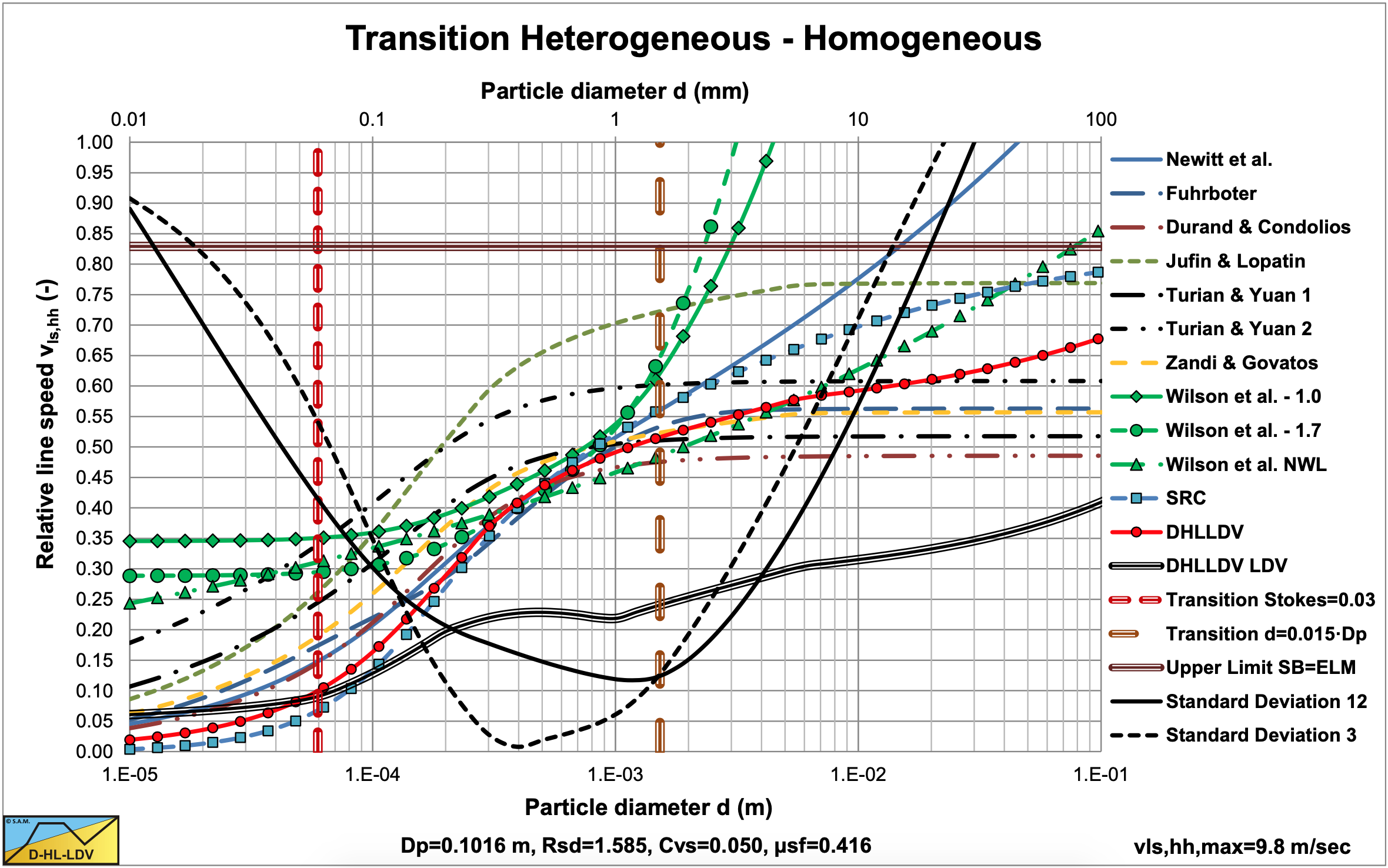
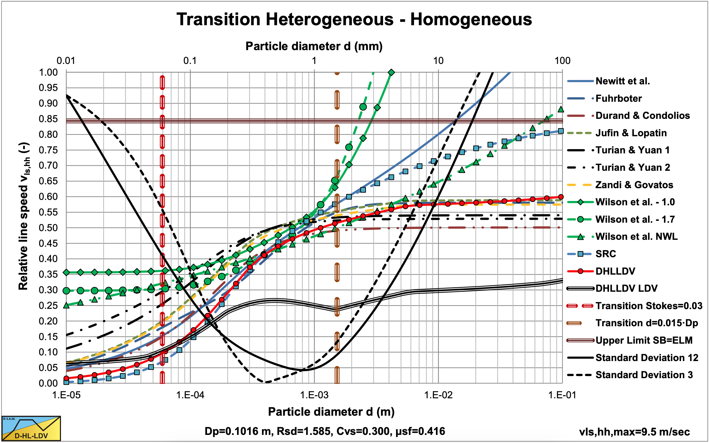
Most models are close for medium sized particles for higher concentrations. The Turian & Yuan 2 and the Jufin & Lopatin models depend on the concentration as can be seen clearly in the figures. The SRC and DHLLDV Framework match closely up to a particle diameter of about 1 mm. The Wilson et al. models matches both models for particle diameters close to 1 mm.

9.2.14.11 A 0.2032 m Diameter Pipe (8 inch)

Figure 9.2-11: The transition line speed He-Ho for D_p=0.2032 m and C_v=0.05

Figure 9.2-12: The transition line speed He-Ho for D_p=0.2032 m and C_v=0.30

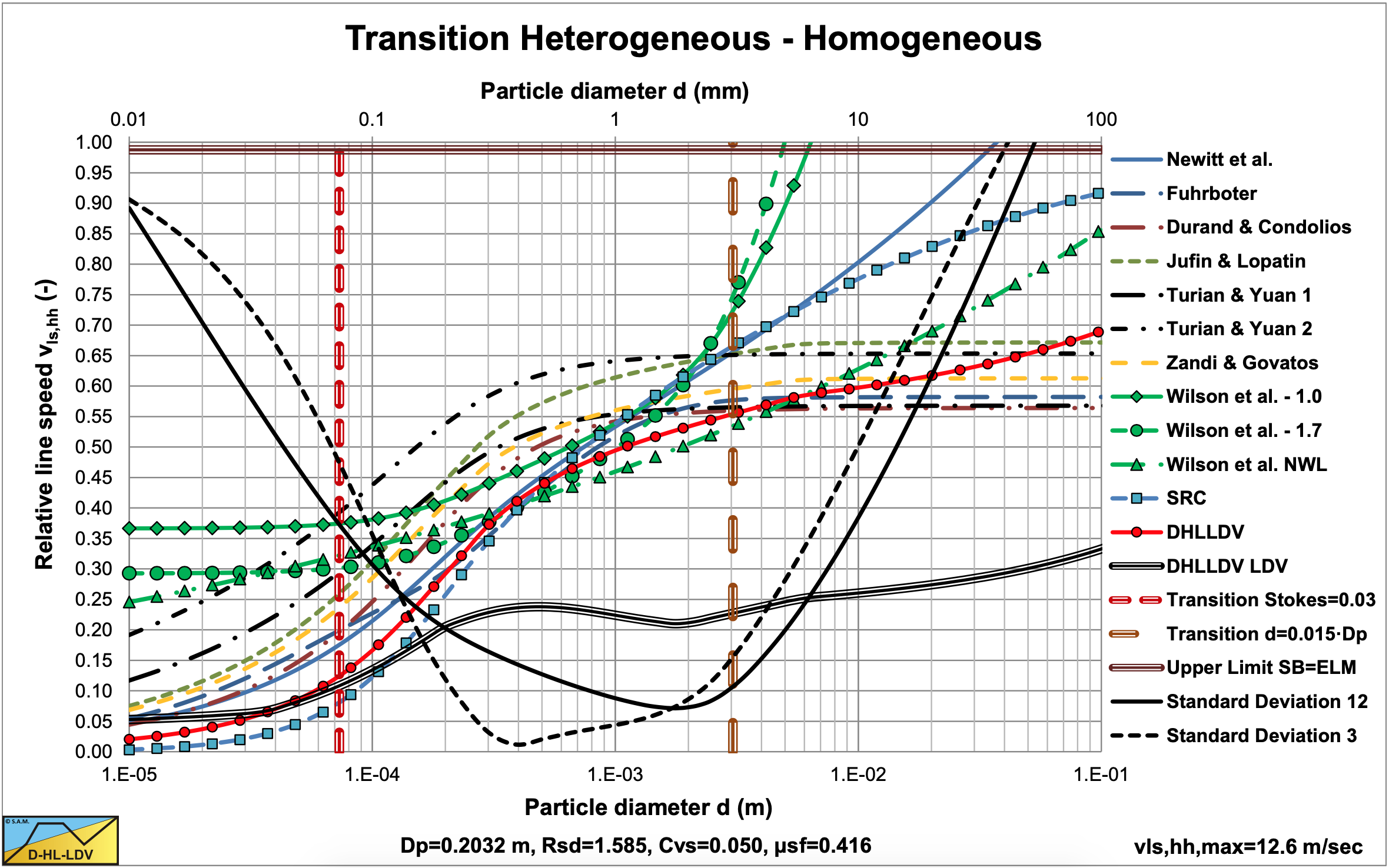
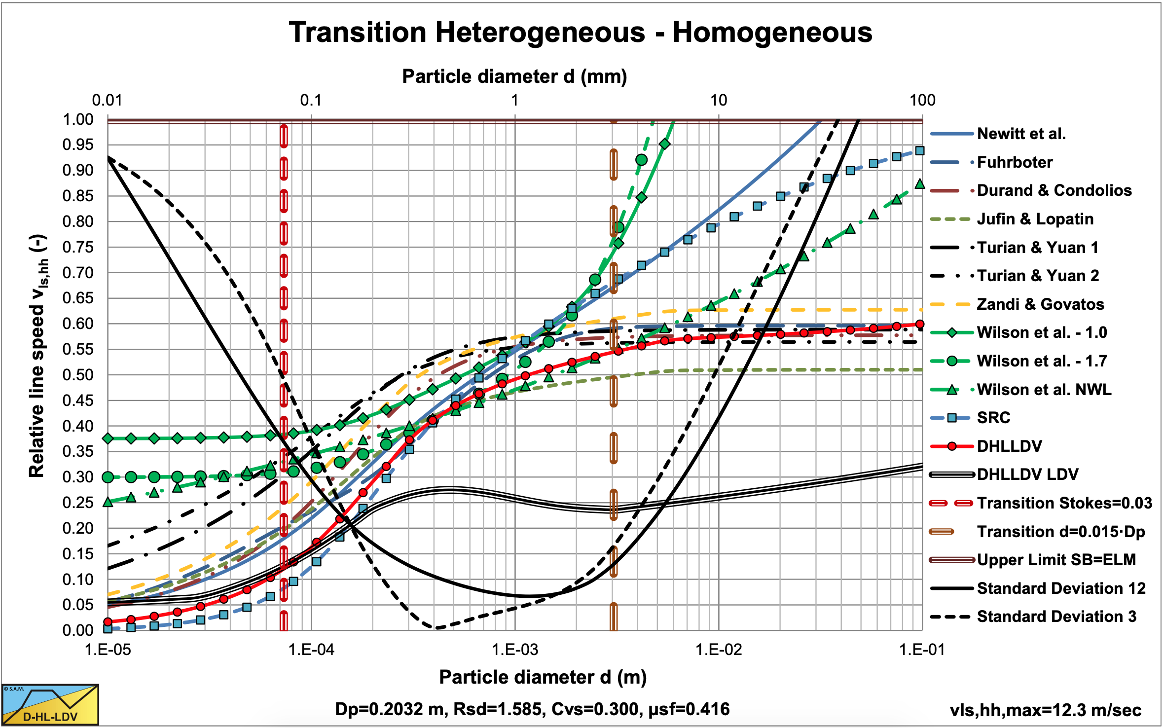
Most models are close for medium sized particles for higher concentrations. The Turian & Yuan 2 and the Jufin & Lopatin models depend on the concentration as can be seen clearly in the figures. The SRC and DHLLDV Framework match closely up to a particle diameter of about 0.6 mm. The Wilson et al. models matches both models for particle diameters close to 1 mm.

9.2.14.12 A 0.4064 m Diameter Pipe (16 inch)

Figure 9.2-13: The transition line speed He-Ho for D_p=0.4064 m and C_v=0.05

Figure 9.2-14: The transition line speed He-Ho for D_p=0.4064 m and C_v=0.30

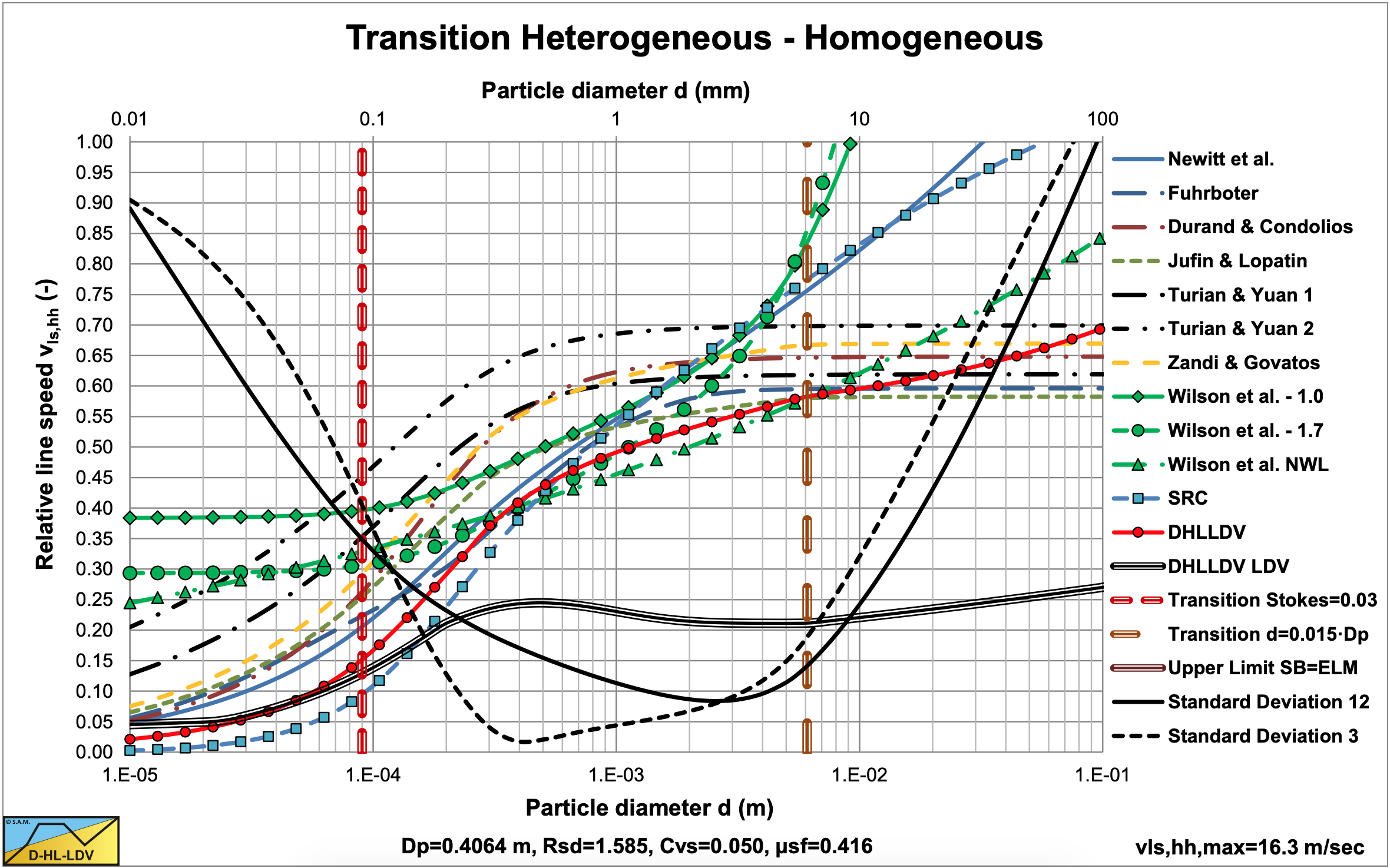
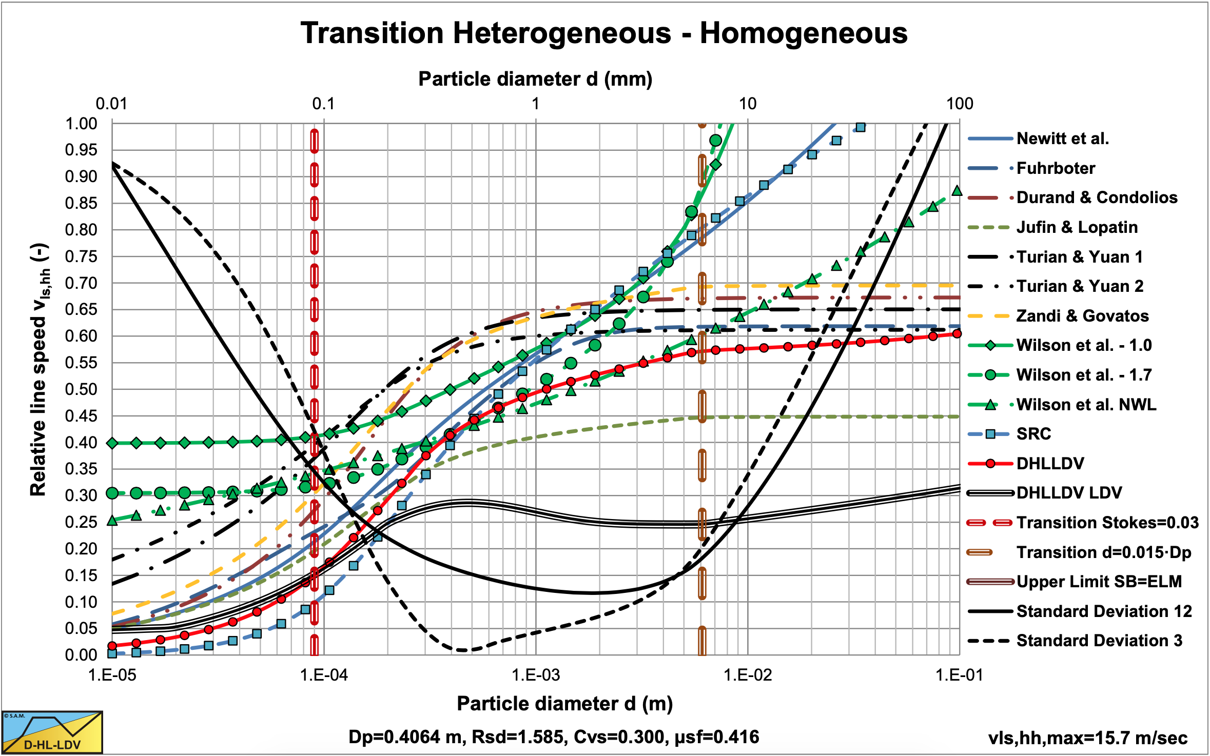
The models start to deviate strongly. Durand & Condolios, Zandi & Govatos and Turian & Yuan 1 and 2 give high transition velocities. Fuhrboter, Newitt et al. and Wilson et al. -1.0 medium transition velocities, while DHLLDV, SRC (small particles), Wilson et al. -1.7 and Jufin & Lopatin (medium concentrations) give low transition velocities.

9.2.14.13 A 0.762 m Diameter Pipe (30 inch)

Figure 9.2-15: The transition line speed He-Ho for D_p=0.762 m and C_v=0.05

Figure 9.2-16: The transition line speed He-Ho for D_p=0.762 m and C_v=0.30

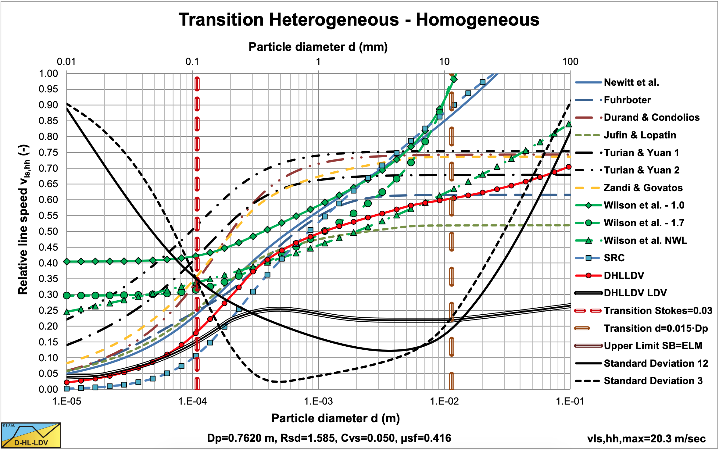
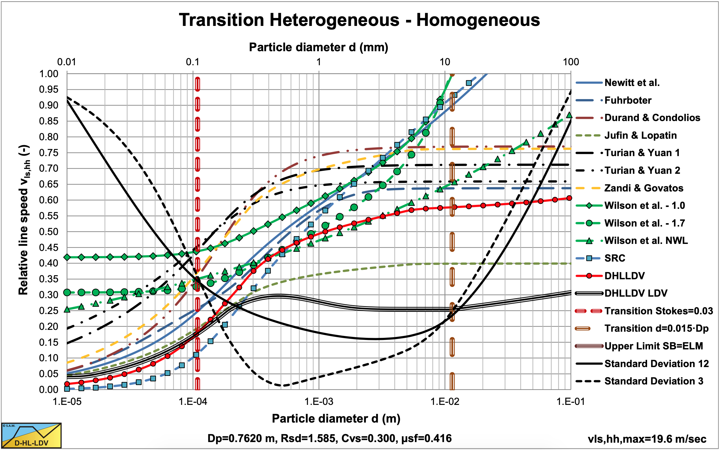
The models deviate strongly. Durand & Condolios, Zandi & Govatos and Turian & Yuan 1 and 2 give high transition velocities. Fuhrboter, Newitt et al. and Wilson et al. -1.0 medium transition velocities, while DHLLDV, SRC (small particles), Wilson et al. -1.7 and Jufin & Lopatin (medium concentrations) give low transition velocities.

9.2.14.14 A 1.2 m Diameter Pipe

Figure 9.2-17: The transition line speed He-Ho for D_p=1.2 m and C_v=0.05

Figure 9.2-18: The transition line speed He-Ho for D_p=1.2 m and C_v=0.30

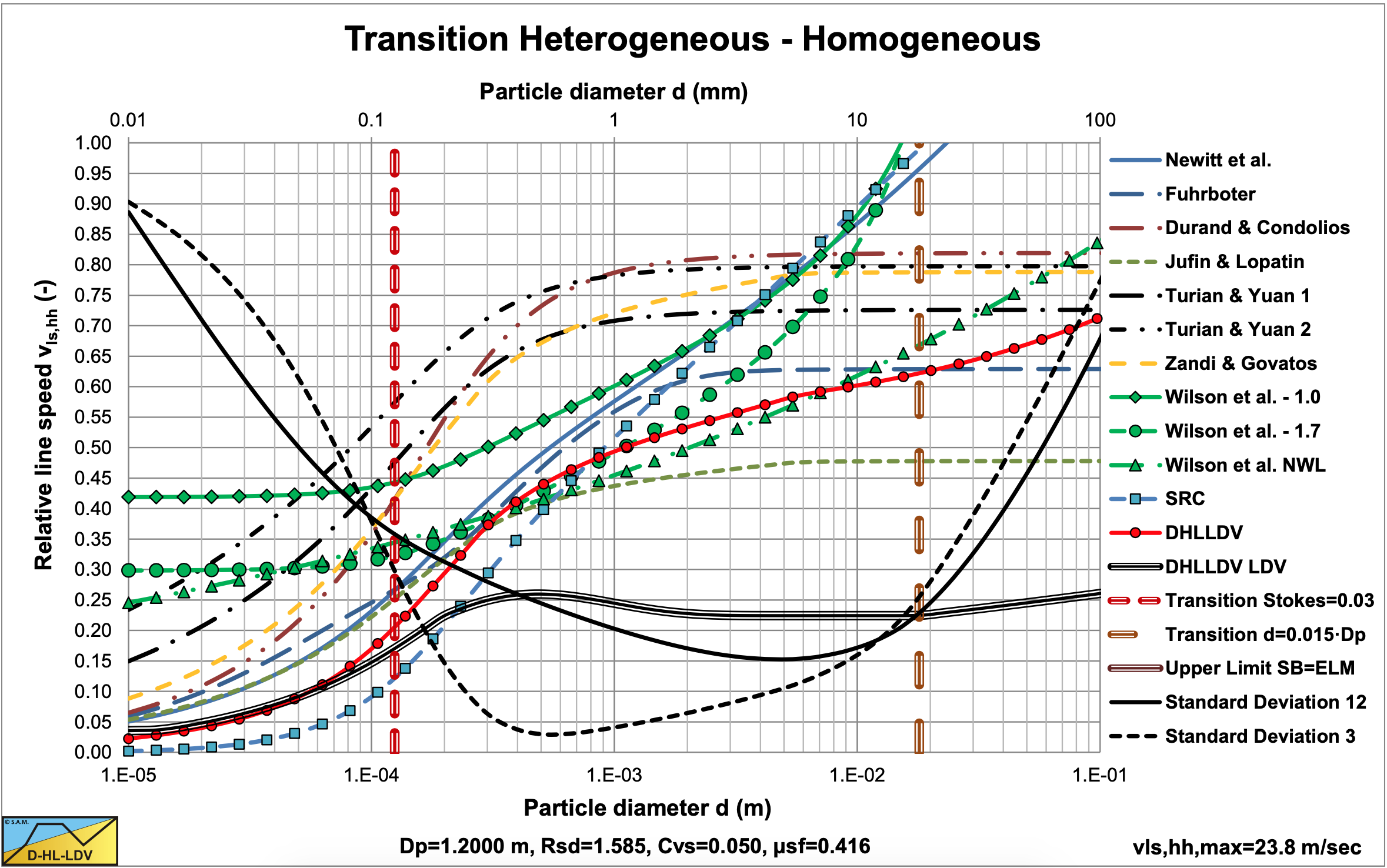
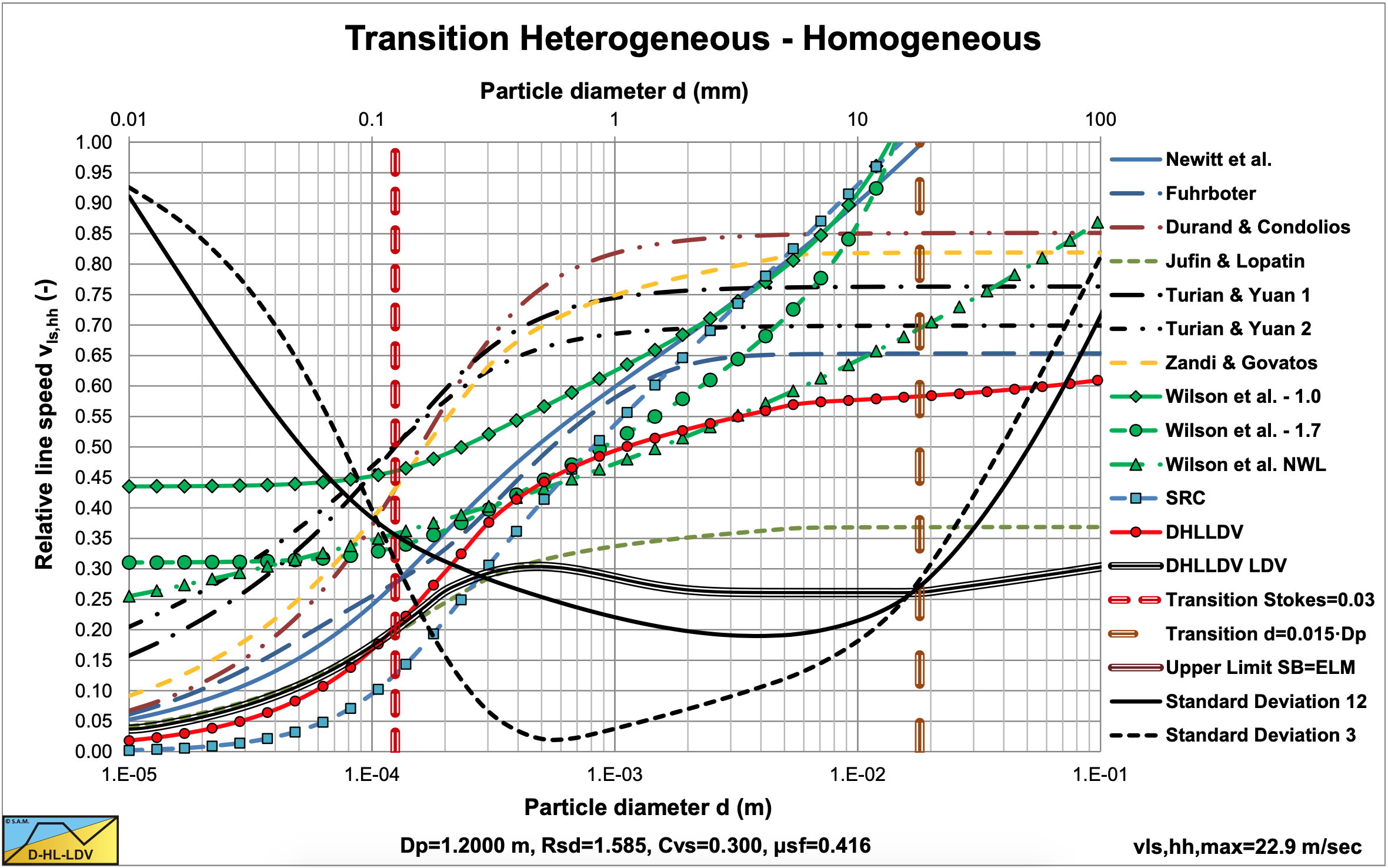
The models deviate strongly. Durand & Condolios, Zandi & Govatos and Turian & Yuan 1 and 2 give high transition velocities. Fuhrboter, Newitt et al. and Wilson et al. -1.0 medium transition velocities, while DHLLDV, SRC (small particles), Wilson et al. -1.7 and Jufin & Lopatin (medium concentrations) give low transition velocities.

9.2.15 Conclusions & Discussion Heterogeneous-Homogeneous Transition

The transition velocity of the heterogeneous regime equation with the ELM equation seems to be a good indicator for comparing the different models. A requirement is of course that the heterogeneous component can be isolated. The hydraulic gradient or head losses can be easily determined at the transition velocity, since the ELM is valid in this intersection point. The solids effect of the hydraulic gradient or head losses is proportional to the transition velocity squared.

When interpreting the graphs, one has to consider the operational line speeds for the pipe diameter considered. For example in Figure 9.2-17 and Figure 9.2-18 the maximum line speeds are 26.3 m/s and 24.6 m/s (the full vertical scale). With a maximum Limit Deposit Velocity of 6-7 m/s and a maximum line speed of about 9 m/s, the operational line speed will be in the range of 0.25 to 0.4 on the vertical axis. If the relative transition velocity is below 0.25 the slurry transport will be in the homogeneous regime, following the ELM or related model. If the relative transition velocity is above 0.4 the slurry transport will probably be a fixed or sliding bed. In between there will be heterogeneous or pseudo homogeneous transport.

Models are based on the terminal settling velocity or models are based on the particle Froude number. The difference between the two groups is, that the terminal settling velocity continuously increases with the particle diameter, while the particle Froude number and the particle drag coefficient have a constant asymptotic value for large particle diameters. So models from the first group tend to overestimate the transition line speed for large particles. This is however not surprising, since both Newitt et al. (1955), SRC and Wilson et al. (1992) use a 2LM or sliding bed model for this case, so the large particle part of the curves is not relevant.

In general one can say that the transition line speed is proportional to the pipe diameter with a power of 0.3 to 0.4, based on the Wilson et al. (1992) models, the SRC model and the DHLLDV Framework.

In general one can say that the transition line speed depends weakly on the spatial concentration.

In general one can say that there is no or hardly no influence of the sliding friction coefficient on the transition velocity of the heterogeneous and the homogeneous regimes.

In general one can say that there is a weak or no direct dependency of the transition velocity of the heterogeneous and the homogeneous regimes on the relative submerged density. Some models give a weak indirect dependency on the particle Froude number.

In general one can say that the more negative the power of the line speed in the heterogeneous hydraulic gradient equation, the smaller the transition velocity between the regimes. One has to take this into account interpreting the graphs.

Based on the amount of experimental data, the SRC model and the Wilson et al. model seem to be the most reliable. The DHLLDV Framework is close to these models for medium sized particles, although DHLLDV is based on potential and kinetic energy losses, while both SRC and Wilson et al. are based on a diminishing bed with increasing line speed.

For the range of operational line speeds, particles smaller than 0.2 mm will usually behave according to ELM or related models, while large particles will behave according to a fixed or sliding bed or according to the sliding flow regime.