3.5: How to choose a neural network's hyper-parameters?

Up until now I haven't explained how I've been choosing values for hyper-parameters such as the learning rate, \(η\), the regularization parameter, \(λ\), and so on. I've just been supplying values which work pretty well. In practice, when you're using neural nets to attack a problem, it can be difficult to find good hyper-parameters. Imagine, for example, that we've just been introduced to the MNIST problem, and have begun working on it, knowing nothing at all about what hyper-parameters to use. Let's suppose that by good fortune in our first experiments we choose many of the hyper-parameters in the same way as was done earlier this chapter: 30 hidden neurons, a mini-batch size of \(10\), training for \(30\) epochs using the cross-entropy. But we choose a learning rate \(η=10.0\) and regularization parameter \(λ=1000.0\). Here's what I saw on one such run:

>>> import mnist_loader
>>> training_data, validation_data, test_data = \
... mnist_loader.load_data_wrapper()
>>> import network2
>>> net = network2.Network([784, 30, 10])
>>> net.SGD(training_data, 30, 10, 10.0, lmbda = 1000.0,
... evaluation_data=validation_data, monitor_evaluation_accuracy=True)
Epoch 0 training complete
Accuracy on evaluation data: 1030 / 10000

Epoch 1 training complete
Accuracy on evaluation data: 990 / 10000

Epoch 2 training complete
Accuracy on evaluation data: 1009 / 10000

...

Epoch 27 training complete
Accuracy on evaluation data: 1009 / 10000

Epoch 28 training complete
Accuracy on evaluation data: 983 / 10000

Epoch 29 training complete
Accuracy on evaluation data: 967 / 10000

Our classification accuracies are no better than chance! Our network is acting as a random noise generator!

"Well, that's easy to fix," you might say, "just decrease the learning rate and regularization hyper-parameters". Unfortunately, you don't a priori know those are the hyper-parameters you need to adjust. Maybe the real problem is that our \(30\) hidden neuron network will never work well, no matter how the other hyper-parameters are chosen? Maybe we really need at least \(100\) hidden neurons? Or \(300\) hidden neurons? Or multiple hidden layers? Or a different approach to encoding the output? Maybe our network is learning, but we need to train for more epochs? Maybe the mini-batches are too small? Maybe we'd do better switching back to the quadratic cost function? Maybe we need to try a different approach to weight initialization? And so on, on and on and on. It's easy to feel lost in hyper-parameter space. This can be particularly frustrating if your network is very large, or uses a lot of training data, since you may train for hours or days or weeks, only to get no result. If the situation persists, it damages your confidence. Maybe neural networks are the wrong approach to your problem? Maybe you should quit your job and take up beekeeping?

In this section I explain some heuristics which can be used to set the hyper-parameters in a neural network. The goal is to help you develop a workflow that enables you to do a pretty good job setting hyper-parameters. Of course, I won't cover everything about hyper-parameter optimization. That's a huge subject, and it's not, in any case, a problem that is ever completely solved, nor is there universal agreement amongst practitioners on the right strategies to use. There's always one more trick you can try to eke out a bit more performance from your network. But the heuristics in this section should get you started.

Broad strategy: When using neural networks to attack a new problem the first challenge is to get any non-trivial learning, i.e., for the network to achieve results better than chance. This can be surprisingly difficult, especially when confronting a new class of problem. Let's look at some strategies you can use if you're having this kind of trouble.

Suppose, for example, that you're attacking MNIST for the first time. You start out enthusiastic, but are a little discouraged when your first network fails completely, as in the example above. The way to go is to strip the problem down. Get rid of all the training and validation images except images which are 0s or 1s. Then try to train a network to distinguish 0s from 1s. Not only is that an inherently easier problem than distinguishing all ten digits, it also reduces the amount of training data by \(80\) percent, speeding up training by a factor of \(5\). That enables much more rapid experimentation, and so gives you more rapid insight into how to build a good network.

You can further speed up experimentation by stripping your network down to the simplest network likely to do meaningful learning. If you believe a [784, 10] network can likely do better-than-chance classification of MNIST digits, then begin your experimentation with such a network. It'll be much faster than training a [784, 30, 10] network, and you can build back up to the latter.

You can get another speed up in experimentation by increasing the frequency of monitoring. In network2.py we monitor performance at the end of each training epoch. With \(50,000\) images per epoch, that means waiting a little while - about ten seconds per epoch, on my laptop, when training a [784, 30, 10] network - before getting feedback on how well the network is learning. Of course, ten seconds isn't very long, but if you want to trial dozens of hyper-parameter choices it's annoying, and if you want to trial hundreds or thousands of choices it starts to get debilitating. We can get feedback more quickly by monitoring the validation accuracy more often, say, after every \(1,000\) training images. Furthermore, instead of using the full \(10,000\) image validation set to monitor performance, we can get a much faster estimate using just \(100\) validation images. All that matters is that the network sees enough images to do real learning, and to get a pretty good rough estimate of performance. Of course, our program network2.py doesn't currently do this kind of monitoring. But as a kludge to achieve a similar effect for the purposes of illustration, we'll strip down our training data to just the first \(1,000\) MNIST training images. Let's try it and see what happens. (To keep the code below simple I haven't implemented the idea of using only \(0\) and \(1\) images. Of course, that can be done with just a little more work.)

>>> net = network2.Network([784, 10])
>>> net.SGD(training_data[:1000], 30, 10, 10.0, lmbda = 1000.0, \
... evaluation_data=validation_data[:100], \
... monitor_evaluation_accuracy=True)
Epoch 0 training complete
Accuracy on evaluation data: 10 / 100

Epoch 1 training complete
Accuracy on evaluation data: 10 / 100

Epoch 2 training complete
Accuracy on evaluation data: 10 / 100
...

We're still getting pure noise! But there's a big win: we're now getting feedback in a fraction of a second, rather than once every ten seconds or so. That means you can more quickly experiment with other choices of hyper-parameter, or even conduct experiments trialling many different choices of hyper-parameter nearly simultaneously.

In the above example I left \(λ\) as \(λ=1000.0\), as we used earlier. But since we changed the number of training examples we should really change \(λ\) to keep the weight decay the same. That means changing \(λ\) to \(20.0\). If we do that then this is what happens:

>>> net = network2.Network([784, 10])
>>> net.SGD(training_data[:1000], 30, 10, 10.0, lmbda = 20.0, \
... evaluation_data=validation_data[:100], \
... monitor_evaluation_accuracy=True)
Epoch 0 training complete
Accuracy on evaluation data: 12 / 100

Epoch 1 training complete
Accuracy on evaluation data: 14 / 100

Epoch 2 training complete
Accuracy on evaluation data: 25 / 100

Epoch 3 training complete
Accuracy on evaluation data: 18 / 100
...

Ahah! We have a signal. Not a terribly good signal, but a signal nonetheless. That's something we can build on, modifying the hyper-parameters to try to get further improvement. Maybe we guess that our learning rate needs to be higher. (As you perhaps realize, that's a silly guess, for reasons we'll discuss shortly, but please bear with me.) So to test our guess we try dialing \(η\) up to \(100.0\):

>>> net = network2.Network([784, 10])
>>> net.SGD(training_data[:1000], 30, 10, 100.0, lmbda = 20.0, \
... evaluation_data=validation_data[:100], \
... monitor_evaluation_accuracy=True)
Epoch 0 training complete
Accuracy on evaluation data: 10 / 100

Epoch 1 training complete
Accuracy on evaluation data: 10 / 100

Epoch 2 training complete
Accuracy on evaluation data: 10 / 100

Epoch 3 training complete
Accuracy on evaluation data: 10 / 100

...

That's no good! It suggests that our guess was wrong, and the problem wasn't that the learning rate was too low. So instead we try dialing ηη down to \(η=1.0\):

>>> net = network2.Network([784, 10])
>>> net.SGD(training_data[:1000], 30, 10, 1.0, lmbda = 20.0, \
... evaluation_data=validation_data[:100], \
... monitor_evaluation_accuracy=True)
Epoch 0 training complete
Accuracy on evaluation data: 62 / 100

Epoch 1 training complete
Accuracy on evaluation data: 42 / 100

Epoch 2 training complete
Accuracy on evaluation data: 43 / 100

Epoch 3 training complete
Accuracy on evaluation data: 61 / 100

...

That's better! And so we can continue, individually adjusting each hyper-parameter, gradually improving performance. Once we've explored to find an improved value for \(η\), then we move on to find a good value for \(λ\). Then experiment with a more complex architecture, say a network with 10 hidden neurons. Then adjust the values for \(η\) and \(λ\) again. Then increase to \(20\) hidden neurons. And then adjust other hyper-parameters some more. And so on, at each stage evaluating performance using our held-out validation data, and using those evaluations to find better and better hyper-parameters. As we do so, it typically takes longer to witness the impact due to modifications of the hyper-parameters, and so we can gradually decrease the frequency of monitoring.

This all looks very promising as a broad strategy. However, I want to return to that initial stage of finding hyper-parameters that enable a network to learn anything at all. In fact, even the above discussion conveys too positive an outlook. It can be immensely frustrating to work with a network that's learning nothing. You can tweak hyper-parameters for days, and still get no meaningful response. And so I'd like to re-emphasize that during the early stages you should make sure you can get quick feedback from experiments. Intuitively, it may seem as though simplifying the problem and the architecture will merely slow you down. In fact, it speeds things up, since you much more quickly find a network with a meaningful signal. Once you've got such a signal, you can often get rapid improvements by tweaking the hyper-parameters. As with many things in life, getting started can be the hardest thing to do.

Okay, that's the broad strategy. Let's now look at some specific recommendations for setting hyper-parameters. I will focus on the learning rate, \(η\), the L2 regularization parameter, \(λ\), and the mini-batch size. However, many of the remarks apply also to other hyper-parameters, including those associated to network architecture, other forms of regularization, and some hyper-parameters we'll meet later in the book, such as the momentum co-efficient.

Learning rate: Suppose we run three MNIST networks with three different learning rates, \(η=0.025\), \(η=0.25\) and \(η=2.5\), respectively. We'll set the other hyper-parameters as for the experiments in earlier sections, running over \(30\) epochs, with a mini-batch size of \(10\), and with \(λ=5.0\). We'll also return to using the full \(50,000\) training images. Here's a graph showing the behaviour of the training cost as we train*

*The graph was generated by multiple_eta.py.:

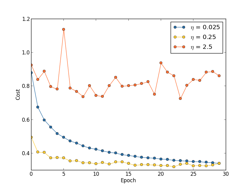
With \(η=0.025\) the cost decreases smoothly until the final epoch. With \(η=0.25\) the cost initially decreases, but after about \(20\) epochs it is near saturation, and thereafter most of the changes are merely small and apparently random oscillations. Finally, with \(η=2.5\) the cost makes large oscillations right from the start. To understand the reason for the oscillations, recall that stochastic gradient descent is supposed to step us gradually down into a valley of the cost function,

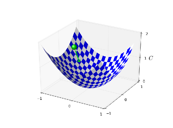
However, if \(η\) is too large then the steps will be so large that they may actually overshoot the minimum, causing the algorithm to climb up out of the valley instead. That's likely*

*This picture is helpful, but it's intended as an intuition-building illustration of what may go on, not as a complete, exhaustive explanation. Briefly, a more complete explanation is as follows: gradient descent uses a first-order approximation to the cost function as a guide to how to decrease the cost. For large \(η\), higher-order terms in the cost function become more important, and may dominate the behaviour, causing gradient descent to break down. This is especially likely as we approach minima and quasi-minima of the cost function, since near such points the gradient becomes small, making it easier for higher-order terms to dominate behaviour. what's causing the cost to oscillate when \(η=2.5\). When we choose \(η=0.25\) the initial steps do take us toward a minimum of the cost function, and it's only once we get near that minimum that we start to suffer from the overshooting problem. And when we choose \(η=0.025\) we don't suffer from this problem at all during the first \(30\) epochs. Of course, choosing ηη so small creates another problem, namely, that it slows down stochastic gradient descent. An even better approach would be to start with \(η=0.25\), train for \(20\) epochs, and then switch to \(η=0.025\). We'll discuss such variable learning rate schedules later. For now, though, let's stick to figuring out how to find a single good value for the learning rate, \(η\).

With this picture in mind, we can set ηη as follows. First, we estimate the threshold value for ηη at which the cost on the training data immediately begins decreasing, instead of oscillating or increasing. This estimate doesn't need to be too accurate. You can estimate the order of magnitude by starting with \(η=0.01\). If the cost decreases during the first few epochs, then you should successively try \(η=0.1,1.0,…\) until you find a value for \(η\) where the cost oscillates or increases during the first few epochs. Alternately, if the cost oscillates or increases during the first few epochs when \(η=0.01\), then try \(η=0.001,0.0001,…\) until you find a value for \(η\) where the cost decreases during the first few epochs. Following this procedure will give us an order of magnitude estimate for the threshold value of ηη. You may optionally refine your estimate, to pick out the largest value of \(η\) at which the cost decreases during the first few epochs, say \(η=0.5\) or \(η=0.2\) (there's no need for this to be super-accurate). This gives us an estimate for the threshold value of \(η\).

Obviously, the actual value of \(η\) that you use should be no larger than the threshold value. In fact, if the value of \(η\) is to remain usable over many epochs then you likely want to use a value for \(η\) that is smaller, say, a factor of two below the threshold. Such a choice will typically allow you to train for many epochs, without causing too much of a slowdown in learning.

In the case of the MNIST data, following this strategy leads to an estimate of \(0.1\) for the order of magnitude of the threshold value of ηη. After some more refinement, we obtain a threshold value \(η=0.5\). Following the prescription above, this suggests using \(η=0.25\) as our value for the learning rate. In fact, I found that using \(η=0.5\) worked well enough over \(30\) epochs that for the most part I didn't worry about using a lower value of \(η\).

This all seems quite straightforward. However, using the training cost to pick ηη appears to contradict what I said earlier in this section, namely, that we'd pick hyper-parameters by evaluating performance using our held-out validation data. In fact, we'll use validation accuracy to pick the regularization hyper-parameter, the mini-batch size, and network parameters such as the number of layers and hidden neurons, and so on. Why do things differently for the learning rate? Frankly, this choice is my personal aesthetic preference, and is perhaps somewhat idiosyncratic. The reasoning is that the other hyper-parameters are intended to improve the final classification accuracy on the test set, and so it makes sense to select them on the basis of validation accuracy. However, the learning rate is only incidentally meant to impact the final classification accuracy. Its primary purpose is really to control the step size in gradient descent, and monitoring the training cost is the best way to detect if the step size is too big. With that said, this is a personal aesthetic preference. Early on during learning the training cost usually only decreases if the validation accuracy improves, and so in practice it's unlikely to make much difference which criterion you use.

Use early stopping to determine the number of training epochs: As we discussed earlier in the chapter, early stopping means that at the end of each epoch we should compute the classification accuracy on the validation data. When that stops improving, terminate. This makes setting the number of epochs very simple. In particular, it means that we don't need to worry about explicitly figuring out how the number of epochs depends on the other hyper-parameters. Instead, that's taken care of automatically. Furthermore, early stopping also automatically prevents us from overfitting. This is, of course, a good thing, although in the early stages of experimentation it can be helpful to turn off early stopping, so you can see any signs of overfitting, and use it to inform your approach to regularization.

To implement early stopping we need to say more precisely what it means that the classification accuracy has stopped improving. As we've seen, the accuracy can jump around quite a bit, even when the overall trend is to improve. If we stop the first time the accuracy decreases then we'll almost certainly stop when there are more improvements to be had. A better rule is to terminate if the best classification accuracy doesn't improve for quite some time. Suppose, for example, that we're doing MNIST. Then we might elect to terminate if the classification accuracy hasn't improved during the last ten epochs. This ensures that we don't stop too soon, in response to bad luck in training, but also that we're not waiting around forever for an improvement that never comes.

This no-improvement-in-ten rule is good for initial exploration of MNIST. However, networks can sometimes plateau near a particular classification accuracy for quite some time, only to then begin improving again. If you're trying to get really good performance, the no-improvement-in-ten rule may be too aggressive about stopping. In that case, I suggest using the no-improvement-in-ten rule for initial experimentation, and gradually adopting more lenient rules, as you better understand the way your network trains: no-improvement-in-twenty, no-improvement-in-fifty, and so on. Of course, this introduces a new hyper-parameter to optimize! In practice, however, it's usually easy to set this hyper-parameter to get pretty good results. Similarly, for problems other than MNIST, the no-improvement-in-ten rule may be much too aggressive or not nearly aggressive enough, depending on the details of the problem. However, with a little experimentation it's usually easy to find a pretty good strategy for early stopping.

We haven't used early stopping in our MNIST experiments to date. The reason is that we've been doing a lot of comparisons between different approaches to learning. For such comparisons it's helpful to use the same number of epochs in each case. However, it's well worth modifying network2.py to implement early stopping:

Problem

• Modify network2.py so that it implements early stopping using a no-improvement-in-\(n\) epochs strategy, where \(n\) is a parameter that can be set.
• Can you think of a rule for early stopping other than no-improvement-in-\(n\)? Ideally, the rule should compromise between getting high validation accuracies and not training too long. Add your rule to network2.py, and run three experiments comparing the validation accuracies and number of epochs of training to no-improvement-in-\(10\).

Learning rate schedule: We've been holding the learning rate \(η\) constant. However, it's often advantageous to vary the learning rate. Early on during the learning process it's likely that the weights are badly wrong. And so it's best to use a large learning rate that causes the weights to change quickly. Later, we can reduce the learning rate as we make more fine-tuned adjustments to our weights.

How should we set our learning rate schedule? Many approaches are possible. One natural approach is to use the same basic idea as early stopping. The idea is to hold the learning rate constant until the validation accuracy starts to get worse. Then decrease the learning rate by some amount, say a factor of two or ten. We repeat this many times, until, say, the learning rate is a factor of 1,024 (or 1,000) times lower than the initial value. Then we terminate.

A variable learning schedule can improve performance, but it also opens up a world of possible choices for the learning schedule. Those choices can be a headache - you can spend forever trying to optimize your learning schedule. For first experiments my suggestion is to use a single, constant value for the learning rate. That'll get you a good first approximation. Later, if you want to obtain the best performance from your network, it's worth experimenting with a learning schedule, along the lines I've described*

*A readable recent paper which demonstrates the benefits of variable learning rates in attacking MNIST is Deep, Big, Simple Neural Nets Excel on Handwritten Digit Recognition, by Dan Claudiu Cireșan, Ueli Meier, Luca Maria Gambardella, and Jürgen Schmidhuber (2010).

Exercise

• Modify network2.py so that it implements a learning schedule that: halves the learning rate each time the validation accuracy satisfies the no-improvement-in-\(10\) rule; and terminates when the learning rate has dropped to \(1/128\) of its original value.

The regularization parameter, \(λ\): I suggest starting initially with no regularization \((λ=0.0)\), and determining a value for ηη, as above. Using that choice of \(η\), we can then use the validation data to select a good value for \(λ\). Start by trialling \(λ=1.0\)*

*I don't have a good principled justification for using this as a starting value. If anyone knows of a good principled discussion of where to start with \(λ\), I'd appreciate hearing it ([e-mail])., and then increase or decrease by factors of \(10\), as needed to improve performance on the validation data. Once you've found a good order of magnitude, you can fine tune your value of \(λ\). That done, you should return and re-optimize \(η\) again.

Exercise

• It's tempting to use gradient descent to try to learn good values for hyper-parameters such as \(λ\) and \(η\). Can you think of an obstacle to using gradient descent to determine \(λ\)? Can you think of an obstacle to using gradient descent to determine \(η\)?

How I selected hyper-parameters earlier in this book: If you use the recommendations in this section you'll find that you get values for \(η\) and \(λ\) which don't always exactly match the values I've used earlier in the book. The reason is that the book has narrative constraints that have sometimes made it impractical to optimize the hyper-parameters. Think of all the comparisons we've made of different approaches to learning, e.g., comparing the quadratic and cross-entropy cost functions, comparing the old and new methods of weight initialization, running with and without regularization, and so on. To make such comparisons meaningful, I've usually tried to keep hyper-parameters constant across the approaches being compared (or to scale them in an appropriate way). Of course, there's no reason for the same hyper-parameters to be optimal for all the different approaches to learning, so the hyper-parameters I've used are something of a compromise.

As an alternative to this compromise, I could have tried to optimize the heck out of the hyper-parameters for every single approach to learning. In principle that'd be a better, fairer approach, since then we'd see the best from every approach to learning. However, we've made dozens of comparisons along these lines, and in practice I found it too computationally expensive. That's why I've adopted the compromise of using pretty good (but not necessarily optimal) choices for the hyper-parameters.

Mini-batch size: How should we set the mini-batch size? To answer this question, let's first suppose that we're doing online learning, i.e., that we're using a mini-batch size of \(1\).

The obvious worry about online learning is that using mini-batches which contain just a single training example will cause significant errors in our estimate of the gradient. In fact, though, the errors turn out to not be such a problem. The reason is that the individual gradient estimates don't need to be super-accurate. All we need is an estimate accurate enough that our cost function tends to keep decreasing. It's as though you are trying to get to the North Magnetic Pole, but have a wonky compass that's 10-20 degrees off each time you look at it. Provided you stop to check the compass frequently, and the compass gets the direction right on average, you'll end up at the North Magnetic Pole just fine.

Based on this argument, it sounds as though we should use online learning. In fact, the situation turns out to be more complicated than that. In a problem in the last chapter I pointed out that it's possible to use matrix techniques to compute the gradient update for all examples in a mini-batch simultaneously, rather than looping over them. Depending on the details of your hardware and linear algebra library this can make it quite a bit faster to compute the gradient estimate for a mini-batch of (for example) size \(100\), rather than computing the mini-batch gradient estimate by looping over the \(100\) training examples separately. It might take (say) only \(50\) times as long, rather than \(100\) times as long.

Now, at first it seems as though this doesn't help us that much. With our mini-batch of size \(100\) the learning rule for the weights looks like:

\[ w→w′=w−η\frac{1}{100}\sum_x{∇C_x},\label{100}\tag{100} \]

where the sum is over training examples in the mini-batch. This is versus

\[ w→w′=w−η∇C_x\label{101}\tag{101} \]

for online learning. Even if it only takes \(50\) times as long to do the mini-batch update, it still seems likely to be better to do online learning, because we'd be updating so much more frequently. Suppose, however, that in the mini-batch case we increase the learning rate by a factor \(100\), so the update rule becomes

\[ w→w′=w−η\sum_x{∇C_x}.\label{102}\tag{102} \]

That's a lot like doing \(100\) separate instances of online learning with a learning rate of \(η\). But it only takes \(50\) times as long as doing a single instance of online learning. Of course, it's not truly the same as \(100\) instances of online learning, since in the mini-batch the \(∇C_x's\) are all evaluated for the same set of weights, as opposed to the cumulative learning that occurs in the online case. Still, it seems distinctly possible that using the larger mini-batch would speed things up.

With these factors in mind, choosing the best mini-batch size is a compromise. Too small, and you don't get to take full advantage of the benefits of good matrix libraries optimized for fast hardware. Too large and you're simply not updating your weights often enough. What you need is to choose a compromise value which maximizes the speed of learning. Fortunately, the choice of mini-batch size at which the speed is maximized is relatively independent of the other hyper-parameters (apart from the overall architecture), so you don't need to have optimized those hyper-parameters in order to find a good mini-batch size. The way to go is therefore to use some acceptable (but not necessarily optimal) values for the other hyper-parameters, and then trial a number of different mini-batch sizes, scaling ηη as above. Plot the validation accuracy versus time (as in, real elapsed time, not epoch!), and choose whichever mini-batch size gives you the most rapid improvement in performance. With the mini-batch size chosen you can then proceed to optimize the other hyper-parameters.

Of course, as you've no doubt realized, I haven't done this optimization in our work. Indeed, our implementation doesn't use the faster approach to mini-batch updates at all. I've simply used a mini-batch size of \(10\) without comment or explanation in nearly all examples. Because of this, we could have sped up learning by reducing the mini-batch size. I haven't done this, in part because I wanted to illustrate the use of mini-batches beyond size 11, and in part because my preliminary experiments suggested the speedup would be rather modest. In practical implementations, however, we would most certainly implement the faster approach to mini-batch updates, and then make an effort to optimize the mini-batch size, in order to maximize our overall speed.

Automated techniques: I've been describing these heuristics as though you're optimizing your hyper-parameters by hand. Hand-optimization is a good way to build up a feel for how neural networks behave. However, and unsurprisingly, a great deal of work has been done on automating the process. A common technique is grid search, which systematically searches through a grid in hyper-parameter space. A review of both the achievements and the limitations of grid search (with suggestions for easily-implemented alternatives) may be found in a 2012 paper*

*Random search for hyper-parameter optimization, by James Bergstra and Yoshua Bengio (2012). by James Bergstra and Yoshua Bengio.

Many more sophisticated approaches have also been proposed. I won't review all that work here, but do want to mention a particularly promising 2012 paper which used a Bayesian approach to automatically optimize hyper-parameters*

*Practical Bayesian optimization of machine learning algorithms, by Jasper Snoek, Hugo Larochelle, and Ryan Adams.. The code from the paper is publicly available, and has been used with some success by other researchers.

Summing up: Following the rules-of-thumb I've described won't give you the absolute best possible results from your neural network. But it will likely give you a good start and a basis for further improvements. In particular, I've discussed the hyper-parameters largely independently. In practice, there are relationships between the hyper-parameters. You may experiment with \(η\), feel that you've got it just right, then start to optimize for \(λ\), only to find that it's messing up your optimization for \(η\). In practice, it helps to bounce backward and forward, gradually closing in good values. Above all, keep in mind that the heuristics I've described are rules of thumb, not rules cast in stone. You should be on the lookout for signs that things aren't working, and be willing to experiment. In particular, this means carefully monitoring your network's behaviour, especially the validation accuracy.

The difficulty of choosing hyper-parameters is exacerbated by the fact that the lore about how to choose hyper-parameters is widely spread, across many research papers and software programs, and often is only available inside the heads of individual practitioners. There are many, many papers setting out (sometimes contradictory) recommendations for how to proceed. However, there are a few particularly useful papers that synthesize and distill out much of this lore. Yoshua Bengio has a 2012 paper*

*Practical recommendations for gradient-based training of deep architectures, by Yoshua Bengio (2012). that gives some practical recommendations for using backpropagation and gradient descent to train neural networks, including deep neural nets. Bengio discusses many issues in much more detail than I have, including how to do more systematic hyper-parameter searches. Another good paper is a 1998 paper*

*Efficient BackProp, by Yann LeCun, Léon Bottou, Genevieve Orr and Klaus-Robert Müller (1998) by Yann LeCun, Léon Bottou, Genevieve Orr and Klaus-Robert Müller. Both these papers appear in an extremely useful 2012 book that collects many tricks commonly used in neural nets*

*Neural Networks: Tricks of the Trade, edited by Grégoire Montavon, Geneviève Orr, and Klaus-Robert Müller.. The book is expensive, but many of the articles have been placed online by their respective authors with, one presumes, the blessing of the publisher, and may be located using a search engine.

One thing that becomes clear as you read these articles and, especially, as you engage in your own experiments, is that hyper-parameter optimization is not a problem that is ever completely solved. There's always another trick you can try to improve performance. There is a saying common among writers that books are never finished, only abandoned. The same is also true of neural network optimization: the space of hyper-parameters is so large that one never really finishes optimizing, one only abandons the network to posterity. So your goal should be to develop a workflow that enables you to quickly do a pretty good job on the optimization, while leaving you the flexibility to try more detailed optimizations, if that's important.

The challenge of setting hyper-parameters has led some people to complain that neural networks require a lot of work when compared with other machine learning techniques. I've heard many variations on the following complaint: "Yes, a well-tuned neural network may get the best performance on the problem. On the other hand, I can try a random forest [or SVM or…… insert your own favorite technique] and it just works. I don't have time to figure out just the right neural network." Of course, from a practical point of view it's good to have easy-to-apply techniques. This is particularly true when you're just getting started on a problem, and it may not be obvious whether machine learning can help solve the problem at all. On the other hand, if getting optimal performance is important, then you may need to try approaches that require more specialist knowledge. While it would be nice if machine learning were always easy, there is no a priori reason it should be trivially simple.