10.1: Traffic jams

What causes traffic jams? Sometimes there is an obvious cause, like an accident, a speed trap, or something else that disturbs the flow of traffic. But other times traffic jams appear for no apparent reason.

Agent-based models can help explain spontaneous traffic jams. As an example, I implement a highway simulation based on a model in Mitchell Resnick’s book, Turtles, Termites and Traffic Jams.

Here’s the class that represents the “highway”:

class Highway: 

    def __init__(self, n=10, length=1000, eps=0): 
        self.length = length 
        self.eps = eps 
        
        # create the drivers 
        locs = np.linspace(0, length, n, endpoint=False) 
        self.drivers = [Driver(loc) for loc in locs] 
        
        # and link them up 
        for i in range(n): 
            j = (i+1) % n 
            self.drivers[i].next = self.drivers[j]

n is the number of cars, length is the length of the highway, and eps is the amount of random noise we’ll add to the system.

locs contains the locations of the drivers; the NumPy function linspace creates an array of n locations equally spaced between 0 and length.

The drivers attribute is a list of Driver objects. The for loop links them so each Driver contains a reference to the next. The highway is circular, so the last Driver contains a reference to the first.

During each time step, the Highway moves each of the drivers:

# Highway 

    def step(self): 
        for driver in self.drivers: 
            self.move(driver)

The move method lets the Driver choose its acceleration. Then move computes the updated speed and position. Here’s the implementation:

# Highway 

    def move(self, driver): 
        dist = self.distance(driver) 
        
        # let the driver choose acceleration 
        acc = driver.choose_acceleration(dist) 
        acc = min(acc, self.max_acc) 
        acc = max(acc, self.min_acc) 
        speed = driver.speed + acc 
        
        # add random noise to speed 
        speed *= np.random.uniform(1-self.eps, 1+self.eps) 
        
        # keep it nonnegative and under the speed limit 
        speed = max(speed, 0) 
        speed = min(speed, self.speed_limit) 
        
        # if current speed would collide, stop 
        if speed > dist: 
            speed = 0 
            
        # update speed and loc 
        driver.speed = speed 
        driver.loc += speed

dist is the distance between driver and the next driver ahead. This distance is passed to choose_acceleration, which specifies the behavior of the driver. This is the only decision the driver gets to make; everything else is determined by the “physics” of the simulation.

• acc is acceleration, which is bounded by min_acc and max_acc. In my implementation, cars can accelerate with max_acc=1 and brake with min_acc=-10.
• speed is the old speed plus the requested acceleration, but then we make some adjustments. First, we add random noise to speed, because the world is not perfect. eps determines the magnitude of the relative error; for example, if eps is 0.02, speed is multiplied by a random factor between 0.98 and 1.02.
• Speed is bounded between 0 and speed_limit, which is 40 in my implementation, so cars are not allowed to go backward or speed.
• If the requested speed would cause a collision with the next car, speed is set to 0.
• Finally, we update the speed and loc attributes of driver.

Here’s the definition for the Driver class:

class Driver: 

    def __init__(self, loc, speed=0): 
        self.loc = loc 
        self.speed = speed 
        
    def choose_acceleration(self, dist): 
        return 1

The attributes loc and speed are the location and speed of the driver.

This implementation of choose_acceleration is simple: it always accelerates at the maximum rate.

Since the cars start out equally spaced, we expect them all to accelerate until they reach the speed limit, or until their speed exceeds the space between them. At that point, at least one “collision” will occur, causing some cars to stop.

Figure \(\PageIndex{1}\): Simulation of drivers on a circular highway at three points in time. Squares indicate the position of the drivers; triangles indicate places where one driver has to brake to avoid another.

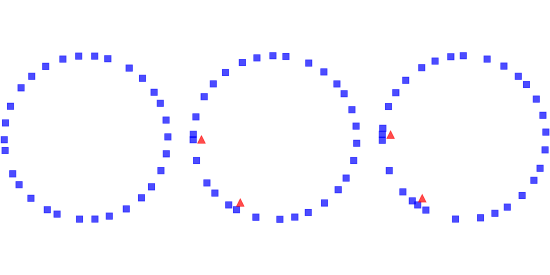
Figure \(\PageIndex{1}\) shows a few steps in this process, starting with 30 cars and eps=0.02. On the left is the configuration after 16 time steps, with the highway mapped to a circle. Because of random noise, some cars are going faster than others, and the spacing has become uneven.

During the next time step (middle) there are two collisions, indicated by the triangles.

During the next time step (right) two cars collide with the stopped cars, and we can see the initial formation of a traffic jam. Once a jam forms, it tends to persist, with additional cars approaching from behind and colliding, and with cars in the front accelerating away.

Under some conditions, the jam itself propagates backwards, as you can see if you watch the animations in the notebook for this chapter.