
2.6: Second-Order Differential and Difference Equations
- Page ID
- 9959

\( \newcommand{\vecs}[1]{\overset { \scriptstyle \rightharpoonup} {\mathbf{#1}} } \)
\( \newcommand{\vecd}[1]{\overset{-\!-\!\rightharpoonup}{\vphantom{a}\smash {#1}}} \)
\( \newcommand{\dsum}{\displaystyle\sum\limits} \)
\( \newcommand{\dint}{\displaystyle\int\limits} \)
\( \newcommand{\dlim}{\displaystyle\lim\limits} \)
\( \newcommand{\id}{\mathrm{id}}\) \( \newcommand{\Span}{\mathrm{span}}\)
( \newcommand{\kernel}{\mathrm{null}\,}\) \( \newcommand{\range}{\mathrm{range}\,}\)
\( \newcommand{\RealPart}{\mathrm{Re}}\) \( \newcommand{\ImaginaryPart}{\mathrm{Im}}\)
\( \newcommand{\Argument}{\mathrm{Arg}}\) \( \newcommand{\norm}[1]{\| #1 \|}\)
\( \newcommand{\inner}[2]{\langle #1, #2 \rangle}\)
\( \newcommand{\Span}{\mathrm{span}}\)
\( \newcommand{\id}{\mathrm{id}}\)
\( \newcommand{\Span}{\mathrm{span}}\)
\( \newcommand{\kernel}{\mathrm{null}\,}\)
\( \newcommand{\range}{\mathrm{range}\,}\)
\( \newcommand{\RealPart}{\mathrm{Re}}\)
\( \newcommand{\ImaginaryPart}{\mathrm{Im}}\)
\( \newcommand{\Argument}{\mathrm{Arg}}\)
\( \newcommand{\norm}[1]{\| #1 \|}\)
\( \newcommand{\inner}[2]{\langle #1, #2 \rangle}\)
\( \newcommand{\Span}{\mathrm{span}}\) \( \newcommand{\AA}{\unicode[.8,0]{x212B}}\)
\( \newcommand{\vectorA}[1]{\vec{#1}} % arrow\)
\( \newcommand{\vectorAt}[1]{\vec{\text{#1}}} % arrow\)
\( \newcommand{\vectorB}[1]{\overset { \scriptstyle \rightharpoonup} {\mathbf{#1}} } \)
\( \newcommand{\vectorC}[1]{\textbf{#1}} \)
\( \newcommand{\vectorD}[1]{\overrightarrow{#1}} \)
\( \newcommand{\vectorDt}[1]{\overrightarrow{\text{#1}}} \)
\( \newcommand{\vectE}[1]{\overset{-\!-\!\rightharpoonup}{\vphantom{a}\smash{\mathbf {#1}}}} \)
\( \newcommand{\vecs}[1]{\overset { \scriptstyle \rightharpoonup} {\mathbf{#1}} } \)
\(\newcommand{\longvect}{\overrightarrow}\)
\( \newcommand{\vecd}[1]{\overset{-\!-\!\rightharpoonup}{\vphantom{a}\smash {#1}}} \)
\(\newcommand{\avec}{\mathbf a}\) \(\newcommand{\bvec}{\mathbf b}\) \(\newcommand{\cvec}{\mathbf c}\) \(\newcommand{\dvec}{\mathbf d}\) \(\newcommand{\dtil}{\widetilde{\mathbf d}}\) \(\newcommand{\evec}{\mathbf e}\) \(\newcommand{\fvec}{\mathbf f}\) \(\newcommand{\nvec}{\mathbf n}\) \(\newcommand{\pvec}{\mathbf p}\) \(\newcommand{\qvec}{\mathbf q}\) \(\newcommand{\svec}{\mathbf s}\) \(\newcommand{\tvec}{\mathbf t}\) \(\newcommand{\uvec}{\mathbf u}\) \(\newcommand{\vvec}{\mathbf v}\) \(\newcommand{\wvec}{\mathbf w}\) \(\newcommand{\xvec}{\mathbf x}\) \(\newcommand{\yvec}{\mathbf y}\) \(\newcommand{\zvec}{\mathbf z}\) \(\newcommand{\rvec}{\mathbf r}\) \(\newcommand{\mvec}{\mathbf m}\) \(\newcommand{\zerovec}{\mathbf 0}\) \(\newcommand{\onevec}{\mathbf 1}\) \(\newcommand{\real}{\mathbb R}\) \(\newcommand{\twovec}[2]{\left[\begin{array}{r}#1 \\ #2 \end{array}\right]}\) \(\newcommand{\ctwovec}[2]{\left[\begin{array}{c}#1 \\ #2 \end{array}\right]}\) \(\newcommand{\threevec}[3]{\left[\begin{array}{r}#1 \\ #2 \\ #3 \end{array}\right]}\) \(\newcommand{\cthreevec}[3]{\left[\begin{array}{c}#1 \\ #2 \\ #3 \end{array}\right]}\) \(\newcommand{\fourvec}[4]{\left[\begin{array}{r}#1 \\ #2 \\ #3 \\ #4 \end{array}\right]}\) \(\newcommand{\cfourvec}[4]{\left[\begin{array}{c}#1 \\ #2 \\ #3 \\ #4 \end{array}\right]}\) \(\newcommand{\fivevec}[5]{\left[\begin{array}{r}#1 \\ #2 \\ #3 \\ #4 \\ #5 \\ \end{array}\right]}\) \(\newcommand{\cfivevec}[5]{\left[\begin{array}{c}#1 \\ #2 \\ #3 \\ #4 \\ #5 \\ \end{array}\right]}\) \(\newcommand{\mattwo}[4]{\left[\begin{array}{rr}#1 \amp #2 \\ #3 \amp #4 \\ \end{array}\right]}\) \(\newcommand{\laspan}[1]{\text{Span}\{#1\}}\) \(\newcommand{\bcal}{\cal B}\) \(\newcommand{\ccal}{\cal C}\) \(\newcommand{\scal}{\cal S}\) \(\newcommand{\wcal}{\cal W}\) \(\newcommand{\ecal}{\cal E}\) \(\newcommand{\coords}[2]{\left\{#1\right\}_{#2}}\) \(\newcommand{\gray}[1]{\color{gray}{#1}}\) \(\newcommand{\lgray}[1]{\color{lightgray}{#1}}\) \(\newcommand{\rank}{\operatorname{rank}}\) \(\newcommand{\row}{\text{Row}}\) \(\newcommand{\col}{\text{Col}}\) \(\renewcommand{\row}{\text{Row}}\) \(\newcommand{\nul}{\text{Nul}}\) \(\newcommand{\var}{\text{Var}}\) \(\newcommand{\corr}{\text{corr}}\) \(\newcommand{\len}[1]{\left|#1\right|}\) \(\newcommand{\bbar}{\overline{\bvec}}\) \(\newcommand{\bhat}{\widehat{\bvec}}\) \(\newcommand{\bperp}{\bvec^\perp}\) \(\newcommand{\xhat}{\widehat{\xvec}}\) \(\newcommand{\vhat}{\widehat{\vvec}}\) \(\newcommand{\uhat}{\widehat{\uvec}}\) \(\newcommand{\what}{\widehat{\wvec}}\) \(\newcommand{\Sighat}{\widehat{\Sigma}}\) \(\newcommand{\lt}{<}\) \(\newcommand{\gt}{>}\) \(\newcommand{\amp}{&}\) \(\definecolor{fillinmathshade}{gray}{0.9}\)With our understanding of the functions \(e^x\), \(e^{jΘ}\), and the quadratic equation \(z^2 + \frac b a z + \frac c a =0\), we can undertake a rudimentary study of differential and difference equations.
Differential Equations
In your study of circuits and systems you will encounter the homogeneous differential equation
\[\frac {d^2} {dt^2} x(t)+a_1\frac d {dt} x(t)+a_2=0 \nonumber \]
Because the function \(e^{st}\) reproduces itself under differentiation, it is plausible to assume that x(t)=est is a solution to the differential equation. Let's try it:
\[\frac {d^2} {dt^2}(e^{st})+a_1\frac d {dt}(e^{st})+a_2(e^{st})=0 \nonumber \]
\[(s^2+a_1s+a_2)e^{st}=0 \nonumber \]
If this equation is to be satisfied for all \(t\), then the polynomial in \(s\) must be zero. Therefore we require
\[s^2+a_1s+a_2=0 \nonumber \]
As we know from our study of this quadratic equation, the solutions are
\[s_{1,2}=−\frac {a_1} 2 ± \frac 1 2 \sqrt{a^2_1−4a_2} \nonumber \]
This means that our assumed solution works, provided \(s=s_1\) or \(s_2\). It is a fundamental result from the theory of differential equations that the most general solution for x(t) is a linear combination of these assumed solutions:
\[x(t)=A_1e^{s_1t}+A_2e^{s_2t} \nonumber \]
If \(a^2_1−4a_2\) is less than zero, then the roots \(s_1\) and \(s_2\) are complex:
\[s_{1,2}=−\frac {a_1} 2 ± j\frac 1 2 \sqrt{4a_2−a^2_1} \nonumber \]
Let's rewrite this solution as
\[s_{1,2}=σ±jω \nonumber \]
where σ and ω are the constants
\[σ=−\frac {a_1} 2 \nonumber \]
\[ω=\frac 1 2 \sqrt{4a_2−a^2_1} \nonumber \]
With this notation, the solution for x(t) is
\[x(t)=A_1e^{σt}e^{jωt}+A_2e^{σt}e^{−jωt} \nonumber \]
If this solution is to be real, then the two terms on the right-hand side must be complex conjugates. This means that \(A_2=A^∗_1\) and the solution for x(t) is
\[x(t)=A_1e^{σt}e^{jωt}+A^∗_1e^{σt}e^{−Jωt} = 2\mathrm{Re} \{A_1e^{σt} e^{jωt}\} \nonumber \]
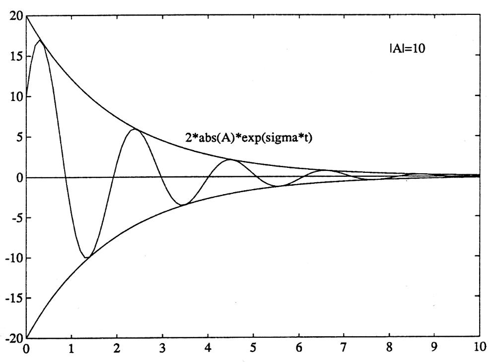
The constant \(A_1\) may be written as \(A_1=|A|e^{jφ}\). Then the solution for x(t) is
\[x(t)=2|A|e^{σt}\cos(ωt+φ) \nonumber \]
This “damped cosinusoidal solution” is illustrated in the Figure.
Find the general solutions to the following differential equations:
a. \(\frac {d^2} {dt^2} X(t)+2\frac d {dt} x(t)+2=0\)
b. \(\frac {d^2} {dt^2} x(t)+2\frac d {dt} x(t)−2=0\)
c. \(\frac {d^2} {dt^2} x(t)+2=0\)
Difference Equations
In your study of digital filters you will encounter homogeneous difference equations of the form
\[x_n+a_1x_n−1+a_2x_{n−2}=0 \nonumber \]
What this means is that the sequence \(\{x_n\}\) obeys a homogeneous recursion:
\[x_n=−a_1x_{n−1}−a_2x_{n−2} \nonumber \]
A plausible guess at a solution is the geometric sequence \(x_n=z^n\). With this guess, the difference equation produces the result
\[z^n+a_1z^n−1+a_2z^{n−2}=0 \nonumber \]
\[(1+a_1z^{−1}+a_2z^{−2})z^n=0 \nonumber \]
If this guess is to work, then the second-order polynomial on the left-hand side must equal zero:
\[1+a_1z^{−1}+a_2z^{−2}=0 \nonumber \]
\[z^2+a_1z+a_2=0 \nonumber \]
The solutions are
\[z_{1,2}=−\frac {a_1} 2 ± j\frac 1 2 \sqrt{4a_2−a^2_1} = re^{jθ} \nonumber \]
The general solution to the difference equation is a linear combination of the assumed solutions:
\[x_n=A_1z^n_1+A_2(z^∗_1)^n \nonumber \]
\[=A_1z^n_1+A^∗_1(z^∗_1) \nonumber \]
\[=2\mathrm{Re}{A_1z^n_1} \nonumber \]
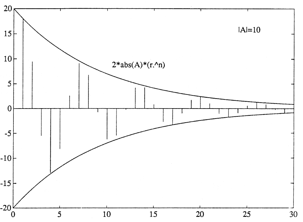
\[=2|A|r^n\cos(θn+φ) \nonumber \]
This general solution is illustrated in the Figure.
Find the general solutions to the following difference equations:
a. x_n+2x_{n−1}+2=0
b. x_n−2x_{n−1}+2=0
c. x_n+2x_{n−2}=0