
2.3: The Function e^jθ and the Unit Circle
- Page ID
- 9956

\( \newcommand{\vecs}[1]{\overset { \scriptstyle \rightharpoonup} {\mathbf{#1}} } \)
\( \newcommand{\vecd}[1]{\overset{-\!-\!\rightharpoonup}{\vphantom{a}\smash {#1}}} \)
\( \newcommand{\dsum}{\displaystyle\sum\limits} \)
\( \newcommand{\dint}{\displaystyle\int\limits} \)
\( \newcommand{\dlim}{\displaystyle\lim\limits} \)
\( \newcommand{\id}{\mathrm{id}}\) \( \newcommand{\Span}{\mathrm{span}}\)
( \newcommand{\kernel}{\mathrm{null}\,}\) \( \newcommand{\range}{\mathrm{range}\,}\)
\( \newcommand{\RealPart}{\mathrm{Re}}\) \( \newcommand{\ImaginaryPart}{\mathrm{Im}}\)
\( \newcommand{\Argument}{\mathrm{Arg}}\) \( \newcommand{\norm}[1]{\| #1 \|}\)
\( \newcommand{\inner}[2]{\langle #1, #2 \rangle}\)
\( \newcommand{\Span}{\mathrm{span}}\)
\( \newcommand{\id}{\mathrm{id}}\)
\( \newcommand{\Span}{\mathrm{span}}\)
\( \newcommand{\kernel}{\mathrm{null}\,}\)
\( \newcommand{\range}{\mathrm{range}\,}\)
\( \newcommand{\RealPart}{\mathrm{Re}}\)
\( \newcommand{\ImaginaryPart}{\mathrm{Im}}\)
\( \newcommand{\Argument}{\mathrm{Arg}}\)
\( \newcommand{\norm}[1]{\| #1 \|}\)
\( \newcommand{\inner}[2]{\langle #1, #2 \rangle}\)
\( \newcommand{\Span}{\mathrm{span}}\) \( \newcommand{\AA}{\unicode[.8,0]{x212B}}\)
\( \newcommand{\vectorA}[1]{\vec{#1}} % arrow\)
\( \newcommand{\vectorAt}[1]{\vec{\text{#1}}} % arrow\)
\( \newcommand{\vectorB}[1]{\overset { \scriptstyle \rightharpoonup} {\mathbf{#1}} } \)
\( \newcommand{\vectorC}[1]{\textbf{#1}} \)
\( \newcommand{\vectorD}[1]{\overrightarrow{#1}} \)
\( \newcommand{\vectorDt}[1]{\overrightarrow{\text{#1}}} \)
\( \newcommand{\vectE}[1]{\overset{-\!-\!\rightharpoonup}{\vphantom{a}\smash{\mathbf {#1}}}} \)
\( \newcommand{\vecs}[1]{\overset { \scriptstyle \rightharpoonup} {\mathbf{#1}} } \)
\(\newcommand{\longvect}{\overrightarrow}\)
\( \newcommand{\vecd}[1]{\overset{-\!-\!\rightharpoonup}{\vphantom{a}\smash {#1}}} \)
\(\newcommand{\avec}{\mathbf a}\) \(\newcommand{\bvec}{\mathbf b}\) \(\newcommand{\cvec}{\mathbf c}\) \(\newcommand{\dvec}{\mathbf d}\) \(\newcommand{\dtil}{\widetilde{\mathbf d}}\) \(\newcommand{\evec}{\mathbf e}\) \(\newcommand{\fvec}{\mathbf f}\) \(\newcommand{\nvec}{\mathbf n}\) \(\newcommand{\pvec}{\mathbf p}\) \(\newcommand{\qvec}{\mathbf q}\) \(\newcommand{\svec}{\mathbf s}\) \(\newcommand{\tvec}{\mathbf t}\) \(\newcommand{\uvec}{\mathbf u}\) \(\newcommand{\vvec}{\mathbf v}\) \(\newcommand{\wvec}{\mathbf w}\) \(\newcommand{\xvec}{\mathbf x}\) \(\newcommand{\yvec}{\mathbf y}\) \(\newcommand{\zvec}{\mathbf z}\) \(\newcommand{\rvec}{\mathbf r}\) \(\newcommand{\mvec}{\mathbf m}\) \(\newcommand{\zerovec}{\mathbf 0}\) \(\newcommand{\onevec}{\mathbf 1}\) \(\newcommand{\real}{\mathbb R}\) \(\newcommand{\twovec}[2]{\left[\begin{array}{r}#1 \\ #2 \end{array}\right]}\) \(\newcommand{\ctwovec}[2]{\left[\begin{array}{c}#1 \\ #2 \end{array}\right]}\) \(\newcommand{\threevec}[3]{\left[\begin{array}{r}#1 \\ #2 \\ #3 \end{array}\right]}\) \(\newcommand{\cthreevec}[3]{\left[\begin{array}{c}#1 \\ #2 \\ #3 \end{array}\right]}\) \(\newcommand{\fourvec}[4]{\left[\begin{array}{r}#1 \\ #2 \\ #3 \\ #4 \end{array}\right]}\) \(\newcommand{\cfourvec}[4]{\left[\begin{array}{c}#1 \\ #2 \\ #3 \\ #4 \end{array}\right]}\) \(\newcommand{\fivevec}[5]{\left[\begin{array}{r}#1 \\ #2 \\ #3 \\ #4 \\ #5 \\ \end{array}\right]}\) \(\newcommand{\cfivevec}[5]{\left[\begin{array}{c}#1 \\ #2 \\ #3 \\ #4 \\ #5 \\ \end{array}\right]}\) \(\newcommand{\mattwo}[4]{\left[\begin{array}{rr}#1 \amp #2 \\ #3 \amp #4 \\ \end{array}\right]}\) \(\newcommand{\laspan}[1]{\text{Span}\{#1\}}\) \(\newcommand{\bcal}{\cal B}\) \(\newcommand{\ccal}{\cal C}\) \(\newcommand{\scal}{\cal S}\) \(\newcommand{\wcal}{\cal W}\) \(\newcommand{\ecal}{\cal E}\) \(\newcommand{\coords}[2]{\left\{#1\right\}_{#2}}\) \(\newcommand{\gray}[1]{\color{gray}{#1}}\) \(\newcommand{\lgray}[1]{\color{lightgray}{#1}}\) \(\newcommand{\rank}{\operatorname{rank}}\) \(\newcommand{\row}{\text{Row}}\) \(\newcommand{\col}{\text{Col}}\) \(\renewcommand{\row}{\text{Row}}\) \(\newcommand{\nul}{\text{Nul}}\) \(\newcommand{\var}{\text{Var}}\) \(\newcommand{\corr}{\text{corr}}\) \(\newcommand{\len}[1]{\left|#1\right|}\) \(\newcommand{\bbar}{\overline{\bvec}}\) \(\newcommand{\bhat}{\widehat{\bvec}}\) \(\newcommand{\bperp}{\bvec^\perp}\) \(\newcommand{\xhat}{\widehat{\xvec}}\) \(\newcommand{\vhat}{\widehat{\vvec}}\) \(\newcommand{\uhat}{\widehat{\uvec}}\) \(\newcommand{\what}{\widehat{\wvec}}\) \(\newcommand{\Sighat}{\widehat{\Sigma}}\) \(\newcommand{\lt}{<}\) \(\newcommand{\gt}{>}\) \(\newcommand{\amp}{&}\) \(\definecolor{fillinmathshade}{gray}{0.9}\)Let's try to extend our definitions of the function \(e^x\) to the argument \(x=jΘ\). Then \(e^{jΘ}\) is the function
\[e^{jθ}=lim_{n→∞}(1+j\frac θ n)^n \nonumber \]
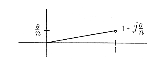
The complex number \(1+j\frac θ n\) is illustrated in the Figure. The radius to the point \(1+j\frac θ n\) is \(r=(1+\frac {θ^2} {n^2})^{1/2}\) and the angle is \(φ=\tan^{−1}\frac θ n\)
This means that the nth power of \(1+j\frac θ n\) has radius \(r^n=(1+\frac {θ^2} {n^2})^{n/2}\) and angle \(nφ=n\;\tan^{−1}\frac θ n\) (Recall our study of powers of z.)
Therefore the complex number \((1+j\frac θ n)^n\) may be written as
\[(1+j\frac θ n)^n=(1+\frac {θ^2} {n^2})^{n/2}[\cos(n\;\tan^{−1}\frac θ n)+j\sin(n\tan^{−1}\frac θ n)] \nonumber \]
For \(n\) large, \((1+\frac {θ^2} {n^2})^{n/2}2≅1\), and \(n\tan^{−1}\frac θ n≅n \frac θ n=θ\). Therefore \((1+j\frac θ n)^n\) is approximately
\[(1+j\frac θ n)^n=1(\cosθ+j\sinθ) \nonumber \]
This finding is consistent with our previous definition of \(e^{jθ}\) !
The series expansion for \(e^{jθ}\) is obtained by evaluating Taylor's formula at \(x=jθ\):
\[e^{jθ}=∑_{n=0}^∞\frac 1 {n!}(jθ)n \nonumber \]
When this series expansion for \(e^{jθ}\) is written out, we have the formula
\[e^{jθ}=∑^∞_{n=0}\frac 1 {(2n)!} (jθ)^{2n}+∑^∞_{n=0}\frac 1 {(2n+1)!}(jθ)^{2n+1} = ∑^∞_{n=0}\frac {(−1)^n} {(2n)!} θ^{2n}+j∑^∞_{n=0}\frac {(−1)^n}{(2n+1)!} θ^{2n+1} \nonumber \]
It is now clear that \(\cosθ\) and \(\sinθ\) have the series expansions
\[\cosθ=∑^∞_{n=0}\frac {(−1)^n} {(2n)!} θ^{2n} \nonumber \]
\[\sinθ=∑_{n=0}^∞\frac {(−1)^n} {(2n+1)!} θ^{2n+1} \nonumber \]
When these infinite sums are truncated at N−1, then we say that we have N-term approximations for \(\cosθ\) and \(\sinθ\):
\[\cosθ≅∑^{N−1}_{n=0} \frac {(−1)^n} {(2n)!} θ^{2n} \nonumber \]
\[\sinθ≅∑_{n=0}^{N−1} \frac {(−1)^n} {(2n+1)!} θ^{2n+1} \nonumber \]
The ten-term approximations to \(\cosθ\) and \(\sinθ\) are plotted over exact expressions for \(\cosθ\) and \(\sinθ\) in the Figure. The approximations are very good over one period \((0≤θ≤2π)\), but they diverge outside this interval. For more accurate approximations over a larger range of θ′s, we would need to use more terms. Or, better yet, we could use the fact that \(cosθ\) and \(sinθ\) are periodic in θ. Then we could subtract as many multiples of \(2π\) as we needed from θ to bring the result into the range \([0,2π]\) and use the ten-term approximations on this new variable. The new variable is called θ-modulo \(2π\).
Write out the first several terms in the series expansions for \(\cosθ\) and \(\sinθ\).
Demo 2.1 (MATLAB)
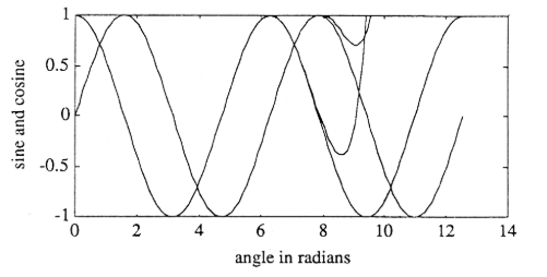
Create a MATLAB file containing the following demo MATLAB program that computes and plots two cycles of \(\cosθ\) and \(\sinθ\) versus θ. You should observe Figure. Note that two cycles take in \(2(2π)\) radians, which is approximately 12 radians.
clg;

j = sqrt(-1);

theta = 0:2*pi/50:4*pi;

s = sin(theta);

c = cos(theta);

plot(theta,s);

elabel('theta in radians');

ylabel('sine and cosine');

hold on

plot(theta,c);

hold off
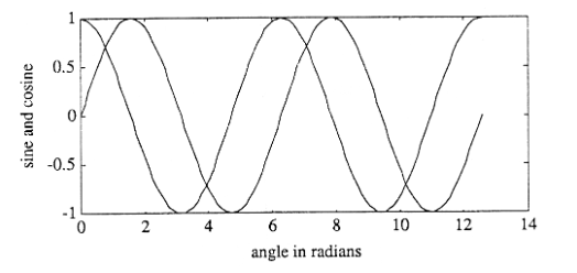
(MATLAB) Write a MATLAB program to compute and plot the ten-term approximations to \(\cosθ\) and \(\sinθ\) for θ running from 0 to \(2(2π)\) in steps of \(2π/50\). Compute and overplot exact expressions for \(\cosθ\) and \(\sinθ\). You should observe a result like the Figure.
The Unit Circle
The unit circle is defined to be the set of all complex numbers z whose magnitudes are 1. This means that all the numbers on the unit circle may be written as \(z=e^{jθ}\). We say that the unit circle consists of all numbers generated by the function \(z=e^{jθ}\) as θ varies from 0 to \(2π\). See below Figure.
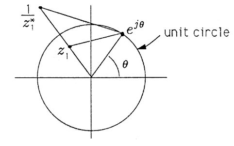
A Fundamental Symmetry
Let's consider the two complex numbers \(z_1\) and \(\frac 1 {z^∗_1}\), illustrated in Figure. We call \(\frac 1 {z^∗_1}\)the “reflection of z through the unit circle” (and vice versa). Note that \(z_1=r_1e^{jθ_1}\) and \(\frac 1 {z^∗_1} = \frac 1 {r_1e^{jθ_1}}\). The complex numbers \(z_1−e^{jθ}\) and \(\frac 1 {z^*_1} −e^{jθ}\) are illustrated in the Figure below. The magnitude squared of each is
\[|z_1−e^{jθ}|^2=(z_1−e^{jθ})(z^∗_1−e^{−jθ}) \nonumber \]
\[|\frac 1 {z^*_1} −e^{jθ}|^2=(\frac 1 {z^*_1−e^{jθ}})(\frac 1 {z_1} −e^{−jθ}) \nonumber \]
The ratio of these magnitudes squared is
\[β^2=\frac {(z_1−e^{jθ})(z^∗_1−e^{−jθ})} {(\frac 1 {z^*_1}−e^{jθ})(\frac 1 {z_1} −e^{−jθ})} \nonumber \]
This ratio may be manipulated to show that it is independent of θ, meaning that the points \(z_1\) and \(\frac 1 {z^∗_1}\) maintain a constant relative distance from every point on the unit circle:
\[β^2=\frac {e^{jθ}(e^{−jθ}z_1−1)(z^∗_1e^{jθ}−1)e^{−jθ}} {\frac {1} {zi} (1−e^{jθ}z^∗_1)(1−z_1e^{−jθ}) \frac 1 z_1} = |z_1|^2 \;,\;\mathrm{independent} \;\mathrm{of}\;θ! \nonumber \]
This result will be of paramount importance to you when you study digital filtering, antenna design, and communication theory.
Write the complex number \(z−e^{jθ}\) as \(re^{jφ}\). What are \(r\) and \(φ\)?