
4.1: The Basic Structure
- Page ID
- 8450

\( \newcommand{\vecs}[1]{\overset { \scriptstyle \rightharpoonup} {\mathbf{#1}} } \)
\( \newcommand{\vecd}[1]{\overset{-\!-\!\rightharpoonup}{\vphantom{a}\smash {#1}}} \)
\( \newcommand{\dsum}{\displaystyle\sum\limits} \)
\( \newcommand{\dint}{\displaystyle\int\limits} \)
\( \newcommand{\dlim}{\displaystyle\lim\limits} \)
\( \newcommand{\id}{\mathrm{id}}\) \( \newcommand{\Span}{\mathrm{span}}\)
( \newcommand{\kernel}{\mathrm{null}\,}\) \( \newcommand{\range}{\mathrm{range}\,}\)
\( \newcommand{\RealPart}{\mathrm{Re}}\) \( \newcommand{\ImaginaryPart}{\mathrm{Im}}\)
\( \newcommand{\Argument}{\mathrm{Arg}}\) \( \newcommand{\norm}[1]{\| #1 \|}\)
\( \newcommand{\inner}[2]{\langle #1, #2 \rangle}\)
\( \newcommand{\Span}{\mathrm{span}}\)
\( \newcommand{\id}{\mathrm{id}}\)
\( \newcommand{\Span}{\mathrm{span}}\)
\( \newcommand{\kernel}{\mathrm{null}\,}\)
\( \newcommand{\range}{\mathrm{range}\,}\)
\( \newcommand{\RealPart}{\mathrm{Re}}\)
\( \newcommand{\ImaginaryPart}{\mathrm{Im}}\)
\( \newcommand{\Argument}{\mathrm{Arg}}\)
\( \newcommand{\norm}[1]{\| #1 \|}\)
\( \newcommand{\inner}[2]{\langle #1, #2 \rangle}\)
\( \newcommand{\Span}{\mathrm{span}}\) \( \newcommand{\AA}{\unicode[.8,0]{x212B}}\)
\( \newcommand{\vectorA}[1]{\vec{#1}} % arrow\)
\( \newcommand{\vectorAt}[1]{\vec{\text{#1}}} % arrow\)
\( \newcommand{\vectorB}[1]{\overset { \scriptstyle \rightharpoonup} {\mathbf{#1}} } \)
\( \newcommand{\vectorC}[1]{\textbf{#1}} \)
\( \newcommand{\vectorD}[1]{\overrightarrow{#1}} \)
\( \newcommand{\vectorDt}[1]{\overrightarrow{\text{#1}}} \)
\( \newcommand{\vectE}[1]{\overset{-\!-\!\rightharpoonup}{\vphantom{a}\smash{\mathbf {#1}}}} \)
\( \newcommand{\vecs}[1]{\overset { \scriptstyle \rightharpoonup} {\mathbf{#1}} } \)
\(\newcommand{\longvect}{\overrightarrow}\)
\( \newcommand{\vecd}[1]{\overset{-\!-\!\rightharpoonup}{\vphantom{a}\smash {#1}}} \)
\(\newcommand{\avec}{\mathbf a}\) \(\newcommand{\bvec}{\mathbf b}\) \(\newcommand{\cvec}{\mathbf c}\) \(\newcommand{\dvec}{\mathbf d}\) \(\newcommand{\dtil}{\widetilde{\mathbf d}}\) \(\newcommand{\evec}{\mathbf e}\) \(\newcommand{\fvec}{\mathbf f}\) \(\newcommand{\nvec}{\mathbf n}\) \(\newcommand{\pvec}{\mathbf p}\) \(\newcommand{\qvec}{\mathbf q}\) \(\newcommand{\svec}{\mathbf s}\) \(\newcommand{\tvec}{\mathbf t}\) \(\newcommand{\uvec}{\mathbf u}\) \(\newcommand{\vvec}{\mathbf v}\) \(\newcommand{\wvec}{\mathbf w}\) \(\newcommand{\xvec}{\mathbf x}\) \(\newcommand{\yvec}{\mathbf y}\) \(\newcommand{\zvec}{\mathbf z}\) \(\newcommand{\rvec}{\mathbf r}\) \(\newcommand{\mvec}{\mathbf m}\) \(\newcommand{\zerovec}{\mathbf 0}\) \(\newcommand{\onevec}{\mathbf 1}\) \(\newcommand{\real}{\mathbb R}\) \(\newcommand{\twovec}[2]{\left[\begin{array}{r}#1 \\ #2 \end{array}\right]}\) \(\newcommand{\ctwovec}[2]{\left[\begin{array}{c}#1 \\ #2 \end{array}\right]}\) \(\newcommand{\threevec}[3]{\left[\begin{array}{r}#1 \\ #2 \\ #3 \end{array}\right]}\) \(\newcommand{\cthreevec}[3]{\left[\begin{array}{c}#1 \\ #2 \\ #3 \end{array}\right]}\) \(\newcommand{\fourvec}[4]{\left[\begin{array}{r}#1 \\ #2 \\ #3 \\ #4 \end{array}\right]}\) \(\newcommand{\cfourvec}[4]{\left[\begin{array}{c}#1 \\ #2 \\ #3 \\ #4 \end{array}\right]}\) \(\newcommand{\fivevec}[5]{\left[\begin{array}{r}#1 \\ #2 \\ #3 \\ #4 \\ #5 \\ \end{array}\right]}\) \(\newcommand{\cfivevec}[5]{\left[\begin{array}{c}#1 \\ #2 \\ #3 \\ #4 \\ #5 \\ \end{array}\right]}\) \(\newcommand{\mattwo}[4]{\left[\begin{array}{rr}#1 \amp #2 \\ #3 \amp #4 \\ \end{array}\right]}\) \(\newcommand{\laspan}[1]{\text{Span}\{#1\}}\) \(\newcommand{\bcal}{\cal B}\) \(\newcommand{\ccal}{\cal C}\) \(\newcommand{\scal}{\cal S}\) \(\newcommand{\wcal}{\cal W}\) \(\newcommand{\ecal}{\cal E}\) \(\newcommand{\coords}[2]{\left\{#1\right\}_{#2}}\) \(\newcommand{\gray}[1]{\color{gray}{#1}}\) \(\newcommand{\lgray}[1]{\color{lightgray}{#1}}\) \(\newcommand{\rank}{\operatorname{rank}}\) \(\newcommand{\row}{\text{Row}}\) \(\newcommand{\col}{\text{Col}}\) \(\renewcommand{\row}{\text{Row}}\) \(\newcommand{\nul}{\text{Nul}}\) \(\newcommand{\var}{\text{Var}}\) \(\newcommand{\corr}{\text{corr}}\) \(\newcommand{\len}[1]{\left|#1\right|}\) \(\newcommand{\bbar}{\overline{\bvec}}\) \(\newcommand{\bhat}{\widehat{\bvec}}\) \(\newcommand{\bperp}{\bvec^\perp}\) \(\newcommand{\xhat}{\widehat{\xvec}}\) \(\newcommand{\vhat}{\widehat{\vvec}}\) \(\newcommand{\uhat}{\widehat{\uvec}}\) \(\newcommand{\what}{\widehat{\wvec}}\) \(\newcommand{\Sighat}{\widehat{\Sigma}}\) \(\newcommand{\lt}{<}\) \(\newcommand{\gt}{>}\) \(\newcommand{\amp}{&}\) \(\definecolor{fillinmathshade}{gray}{0.9}\)Conceptually, a skiplist is a sequence of singly-linked lists \(L_0,\ldots,L_h\). Each list \(L_r\) contains a subset of the items in \(L_{r-1}\). We start with the input list \(L_0\) that contains \(\mathtt{n}\) items and construct \(L_1\) from \(L_0\), \(L_2\) from \(L_1\), and so on. The items in \(L_r\) are obtained by tossing a coin for each element, \(\mathtt{x}\), in \(L_{r-1}\) and including \(\mathtt{x}\) in \(L_r\) if the coin turns up as heads. This process ends when we create a list \(L_r\) that is empty. An example of a skiplist is shown in Figure \(\PageIndex{1}\).
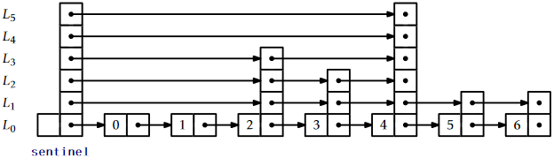
For an element, \(\mathtt{x}\), in a skiplist, we call the height of \(\mathtt{x}\) the largest value \(r\) such that \(\mathtt{x}\) appears in \(L_r\). Thus, for example, elements that only appear in \(L_0\) have height 0. If we spend a few moments thinking about it, we notice that the height of \(\mathtt{x}\) corresponds to the following experiment: Toss a coin repeatedly until it comes up as tails. How many times did it come up as heads? The answer, not surprisingly, is that the expected height of a node is 1. (We expect to toss the coin twice before getting tails, but we don't count the last toss.) The height of a skiplist is the height of its tallest node.
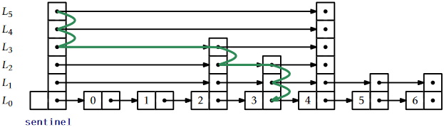
At the head of every list is a special node, called the sentinel, that acts as a dummy node for the list. The key property of skiplists is that there is a short path, called the search path, from the sentinel in \(L_h\) to every node in \(L_0\). Remembering how to construct a search path for a node, \(\mathtt{u}\), is easy (see Figure \(\PageIndex{2}\)) : Start at the top left corner of your skiplist (the sentinel in \(L_h\)) and always go right unless that would overshoot \(\mathtt{u}\), in which case you should take a step down into the list below.
More precisely, to construct the search path for the node \(\mathtt{u}\) in \(L_0\), we start at the sentinel, \(\mathtt{w}\), in \(L_h\). Next, we examine \(\texttt{w.next}\). If \(\texttt{w.next}\) contains an item that appears before \(\mathtt{u}\) in \(L_0\), then we set \(\mathtt{w}=\texttt{w.next}\). Otherwise, we move down and continue the search at the occurrence of \(\mathtt{w}\) in the list \(L_{h-1}\). We continue this way until we reach the predecessor of \(\mathtt{u}\) in \(L_0\).
The following result, which we will prove in Section 4.4, shows that the search path is quite short:
The expected length of the search path for any node, \(\mathtt{u}\), in \(L_0\) is at most \(2\log \mathtt{n} + O(1) = O(\log \mathtt{n})\).
A space-efficient way to implement a skiplist is to define a Node, \(\mathtt{u}\), as consisting of a data value, \(\mathtt{x}\), and an array, \(\mathtt{next}\), of pointers, where \(\mathtt{u.next[i]}\) points to \(\mathtt{u}\)'s successor in the list \(L_{\mathtt{i}}\). In this way, the data, \(\mathtt{x}\), in a node is referenced only once, even though \(\mathtt{x}\) may appear in several lists.
    class Node<T> {
        T x;
        Node<T>[] next;
        Node(T ix, int h) {
            x = ix;
            next = (Node<T>[])Array.newInstance(Node.class, h+1);
        }
        int height() {
            return next.length - 1;
        }
    }
The next two sections of this chapter discuss two different applications of skiplists. In each of these applications, \(L_0\) stores the main structure (a list of elements or a sorted set of elements). The primary difference between these structures is in how a search path is navigated; in particular, they differ in how they decide if a search path should go down into \(L_{r-1}\) or go right within \(L_r\).