3.4: Finite-State Automata
- Page ID
- 6725
\( \newcommand{\vecs}[1]{\overset { \scriptstyle \rightharpoonup} {\mathbf{#1}} } \)
\( \newcommand{\vecd}[1]{\overset{-\!-\!\rightharpoonup}{\vphantom{a}\smash {#1}}} \)
\( \newcommand{\dsum}{\displaystyle\sum\limits} \)
\( \newcommand{\dint}{\displaystyle\int\limits} \)
\( \newcommand{\dlim}{\displaystyle\lim\limits} \)
\( \newcommand{\id}{\mathrm{id}}\) \( \newcommand{\Span}{\mathrm{span}}\)
( \newcommand{\kernel}{\mathrm{null}\,}\) \( \newcommand{\range}{\mathrm{range}\,}\)
\( \newcommand{\RealPart}{\mathrm{Re}}\) \( \newcommand{\ImaginaryPart}{\mathrm{Im}}\)
\( \newcommand{\Argument}{\mathrm{Arg}}\) \( \newcommand{\norm}[1]{\| #1 \|}\)
\( \newcommand{\inner}[2]{\langle #1, #2 \rangle}\)
\( \newcommand{\Span}{\mathrm{span}}\)
\( \newcommand{\id}{\mathrm{id}}\)
\( \newcommand{\Span}{\mathrm{span}}\)
\( \newcommand{\kernel}{\mathrm{null}\,}\)
\( \newcommand{\range}{\mathrm{range}\,}\)
\( \newcommand{\RealPart}{\mathrm{Re}}\)
\( \newcommand{\ImaginaryPart}{\mathrm{Im}}\)
\( \newcommand{\Argument}{\mathrm{Arg}}\)
\( \newcommand{\norm}[1]{\| #1 \|}\)
\( \newcommand{\inner}[2]{\langle #1, #2 \rangle}\)
\( \newcommand{\Span}{\mathrm{span}}\) \( \newcommand{\AA}{\unicode[.8,0]{x212B}}\)
\( \newcommand{\vectorA}[1]{\vec{#1}} % arrow\)
\( \newcommand{\vectorAt}[1]{\vec{\text{#1}}} % arrow\)
\( \newcommand{\vectorB}[1]{\overset { \scriptstyle \rightharpoonup} {\mathbf{#1}} } \)
\( \newcommand{\vectorC}[1]{\textbf{#1}} \)
\( \newcommand{\vectorD}[1]{\overrightarrow{#1}} \)
\( \newcommand{\vectorDt}[1]{\overrightarrow{\text{#1}}} \)
\( \newcommand{\vectE}[1]{\overset{-\!-\!\rightharpoonup}{\vphantom{a}\smash{\mathbf {#1}}}} \)
\( \newcommand{\vecs}[1]{\overset { \scriptstyle \rightharpoonup} {\mathbf{#1}} } \)
\(\newcommand{\longvect}{\overrightarrow}\)
\( \newcommand{\vecd}[1]{\overset{-\!-\!\rightharpoonup}{\vphantom{a}\smash {#1}}} \)
\(\newcommand{\avec}{\mathbf a}\) \(\newcommand{\bvec}{\mathbf b}\) \(\newcommand{\cvec}{\mathbf c}\) \(\newcommand{\dvec}{\mathbf d}\) \(\newcommand{\dtil}{\widetilde{\mathbf d}}\) \(\newcommand{\evec}{\mathbf e}\) \(\newcommand{\fvec}{\mathbf f}\) \(\newcommand{\nvec}{\mathbf n}\) \(\newcommand{\pvec}{\mathbf p}\) \(\newcommand{\qvec}{\mathbf q}\) \(\newcommand{\svec}{\mathbf s}\) \(\newcommand{\tvec}{\mathbf t}\) \(\newcommand{\uvec}{\mathbf u}\) \(\newcommand{\vvec}{\mathbf v}\) \(\newcommand{\wvec}{\mathbf w}\) \(\newcommand{\xvec}{\mathbf x}\) \(\newcommand{\yvec}{\mathbf y}\) \(\newcommand{\zvec}{\mathbf z}\) \(\newcommand{\rvec}{\mathbf r}\) \(\newcommand{\mvec}{\mathbf m}\) \(\newcommand{\zerovec}{\mathbf 0}\) \(\newcommand{\onevec}{\mathbf 1}\) \(\newcommand{\real}{\mathbb R}\) \(\newcommand{\twovec}[2]{\left[\begin{array}{r}#1 \\ #2 \end{array}\right]}\) \(\newcommand{\ctwovec}[2]{\left[\begin{array}{c}#1 \\ #2 \end{array}\right]}\) \(\newcommand{\threevec}[3]{\left[\begin{array}{r}#1 \\ #2 \\ #3 \end{array}\right]}\) \(\newcommand{\cthreevec}[3]{\left[\begin{array}{c}#1 \\ #2 \\ #3 \end{array}\right]}\) \(\newcommand{\fourvec}[4]{\left[\begin{array}{r}#1 \\ #2 \\ #3 \\ #4 \end{array}\right]}\) \(\newcommand{\cfourvec}[4]{\left[\begin{array}{c}#1 \\ #2 \\ #3 \\ #4 \end{array}\right]}\) \(\newcommand{\fivevec}[5]{\left[\begin{array}{r}#1 \\ #2 \\ #3 \\ #4 \\ #5 \\ \end{array}\right]}\) \(\newcommand{\cfivevec}[5]{\left[\begin{array}{c}#1 \\ #2 \\ #3 \\ #4 \\ #5 \\ \end{array}\right]}\) \(\newcommand{\mattwo}[4]{\left[\begin{array}{rr}#1 \amp #2 \\ #3 \amp #4 \\ \end{array}\right]}\) \(\newcommand{\laspan}[1]{\text{Span}\{#1\}}\) \(\newcommand{\bcal}{\cal B}\) \(\newcommand{\ccal}{\cal C}\) \(\newcommand{\scal}{\cal S}\) \(\newcommand{\wcal}{\cal W}\) \(\newcommand{\ecal}{\cal E}\) \(\newcommand{\coords}[2]{\left\{#1\right\}_{#2}}\) \(\newcommand{\gray}[1]{\color{gray}{#1}}\) \(\newcommand{\lgray}[1]{\color{lightgray}{#1}}\) \(\newcommand{\rank}{\operatorname{rank}}\) \(\newcommand{\row}{\text{Row}}\) \(\newcommand{\col}{\text{Col}}\) \(\renewcommand{\row}{\text{Row}}\) \(\newcommand{\nul}{\text{Nul}}\) \(\newcommand{\var}{\text{Var}}\) \(\newcommand{\corr}{\text{corr}}\) \(\newcommand{\len}[1]{\left|#1\right|}\) \(\newcommand{\bbar}{\overline{\bvec}}\) \(\newcommand{\bhat}{\widehat{\bvec}}\) \(\newcommand{\bperp}{\bvec^\perp}\) \(\newcommand{\xhat}{\widehat{\xvec}}\) \(\newcommand{\vhat}{\widehat{\vvec}}\) \(\newcommand{\uhat}{\widehat{\uvec}}\) \(\newcommand{\what}{\widehat{\wvec}}\) \(\newcommand{\Sighat}{\widehat{\Sigma}}\) \(\newcommand{\lt}{<}\) \(\newcommand{\gt}{>}\) \(\newcommand{\amp}{&}\) \(\definecolor{fillinmathshade}{gray}{0.9}\)We have seen how regular expressions can be used to generate languages mechanically. How might languages be recognized mechanically? The question is of interest because if we can mechanically recognize languages like L = {all legal C++ programs that will not go into infinite loops on any input}, then it would be possible to write uber-compilers that can do semantic error-checking like testing for infinite loops, in addition to the syntactic error-checking they currently do.
What formalism might we use to model what it means to recognize a language “mechanically”? We look for inspiration to a language-recognizer with which we are all familiar, and which we’ve already in fact mentioned: a compiler. Consider how a C++ compiler might handle recognizing a legal if statement. Having seen the word if, the compiler will be in a state or phase of its execution where it expects to see a ‘(’; in this state, any other character will put the compiler in a “failure” state. If the compiler does in fact see a ‘(’ next, it will then be in an “expecting a boolean condition” state; if it sees a sequence of symbols that make up a legal boolean condition, it will then be in an “expecting a ‘)’” state; and then “expecting a ‘{’ or a legal statement”; and so on. Thus one can think of the compiler as being in a series of states; on seeing a new input symbol, it moves on to a new state; and this sequence of transitions eventually leads to either a “failure” state (if the if statement is not syntactically correct) or a “success” state (if the if statement is legal). We isolate these three concepts—states, input-inspired transitions from state to state, and “accepting” vs “non-accepting” states— as the key features of a mechanical language-recognizer, and capture them in a model called a finite-state automaton. (Whether this is a successful distillation of the essence of mechanical language recognition remains to be seen; the question will be taken up later in this chapter.)
A finite-state automaton (FSA), then, is a machine which takes, as input, a finite string of symbols from some alphabet Σ. There is a finite set of states in which the machine can find itself. The state it is in before consuming any input is called the start state. Some of the states are accepting or final. If the machine ends in such a state after completely consuming an input string, the string is said to be accepted by the machine. The actual functioning of the machine is described by something called a transition function, which specifies what happens if the machine is in a particular state and looking at a particular input symbol. (“What happens” means “in which state does the machine end up”.)
Example 3.9. Below is a table that describes the transition function of a finite-state automaton with states p, q, and r, on inputs 0 and 1.

The table indicates, for example, that if the FSA were in state p and consumed a 1, it would move to state q.
FSAs actually come in two flavours depending on what properties you require of the transition function. We will look first at a class of FSAs called deterministic finite-state automata (DFAs). In these machines, the current state of the machine and the current input symbol together deter- mine exactly which state the machine ends up in: for every <current state, current input symbol> pair, there is exactly one possible next state for the machine.
Definition 3.5
Formally, a deterministic finite-state automaton M is specified by 5 components: \(M=\left(Q, \Sigma, q_{0}, \delta, F\right)\) where
- Q is a finite set of states;
- Σ is an alphabet called the input alphabet;
- \(q_{0} \in Q\) is a state which is designated as the start state;
- F is a subset of Q; the states in F are states designated as final or accepting states;
- δ is a transition function that takes <state, input symbol> pairs and maps each one to a state: \(\delta : Q \times \Sigma \rightarrow Q\). To say \(\delta(q, a)=q^{\prime}\) means that if the machine is in state q and the input symbol a is consumed, then the machine will move into state q′. The function δ must be a total function, meaning that δ(q,a) must be defined for every state q and every input symbol a. (Recall also that, according to the definition of a function, there can be only one output for any particular input. This means that for any given q and a, δ(q,a) can have only one value. This is what makes the finite-state automaton deterministic: given the current state and input symbol, there is only one possible move the machine can make.)
Example 3.10. The transition function described by the table in the pre- ceding example is that of a DFA. If we take p to be the start state and rto be a final state, then the formal description of the resulting machine is M = ({p,q,r},{0,1},p,δ,{r}), where δ is given by
\(\begin{array}{ll}{\delta(p, 0)=p} & {\delta(p, 1)=q} \\ {\delta(q, 0)=q} & {\delta(q, 1)=r} \\ {\delta(r, 0)=r} & {\delta(r, 1)=r}\end{array}\)
The transition function δ describes only individual steps of the machine as individual input symbols are consumed. However, we will often want to refer to “the state the automaton will be in if it starts in state q and consumes input string w”, where w is a string of input symbols rather than a single symbol. Following the usual practice of using ∗ to designate “0 or more”, we define δ∗(q,w) as a convenient shorthand for “the state that the automaton will be in if it starts in state q and consumes the input stringw”. For any string, it is easy to see, based on δ, what steps the machine will make as those symbols are consumed, and what δ∗(q, w) will be for any q and w. Note that if no input is consumed, a DFA makes no move, and so δ∗(q, ε) = q for any state q.
Example 3.11. Let M be the automaton in the preceding example. Then, for example:
\(\delta^{*}(p, 001)=q,\) since \(\delta(p, 0)=p, \delta(p, 0)=p,\) and \(\delta(p, 1)=q\)
\(\delta^{*}(p, 01000)=q\)
\(\delta^{*}(p, 1111)=r\)
\(\delta^{*}(q, 0010)=r\)
We have divided the states of a DFA into accepting and non-accepting states, with the idea that some strings will be recognized as “legal” by the automaton, and some not. Formally:
Definition 3.6.
Let \(M=\left(Q, \Sigma, q_{0}, \delta, F\right) .\) A string \(w \in \Sigma^{*}\) is accepted by \(M\) iff \(\delta^{*}\left(q_{0}, w\right) \in F\). (Don’t get confused by the notation. Remember, it’s just a shorter and neater way of saying "\(w \in \Sigma^{*}\) is accepted by M if and only if the state that M will end up in if it starts in q0 and consumes w is one of the states in F.”)
The language accepted by M, denoted L(M), is the set of all strings \(w \in \Sigma^{*}\) that are accepted by \(M : L(M)=\left\{w \in \Sigma^{*} | \delta^{*}\left(q_{0}, w\right) \in F\right\}\).
Note that we sometimes use a slightly different phrasing and say that a language L is accepted by some machine M. We don’t mean by this that L and maybe some other strings are accepted by M; we mean L = L(M), i.e. L is exactly the set of strings accepted by M.
It may not be easy, looking at a formal specification of a DFA, to determine what language that automaton accepts. Fortunately, the mathematical description of the automaton \(M=\left(Q, \Sigma, q_{0}, \delta, F\right)\) can be neatly and helpfully captured in a picture called a transition diagram. Consider again the DFA of the two preceding examples. It can be represented pictorially as:

The arrow on the left indicates that p is the start state; double circles indicate that a state is accepting. Looking at this picture, it should be fairly easy to see that the language accepted by the DFA M is L(M) = \(\left\{x \in\{0,1\} * | n_{1}(x) \geq 2\right\}\)
Example 3.12. Find the language accepted by the DFA shown below (and describe it using a regular expression!)
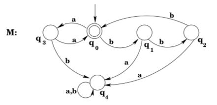
The start state of M is accepting, which means ε ∈ L(M). If M is in state \(q_{0}\), a sequence of two a’s or three b’s will move M back to \(q_{0}\) and hence be accepted. So \(L(M)=L\left((a a | b b b)^{*}\right)\).
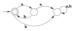
The state \(q_{4}\) in the preceding example is often called a garbage or trap state: it is a non-accepting state which, once reached by the machine, cannot be escaped. It is fairly common to omit such states from transition diagrams. For example, one is likely to see the diagram:

Note that this cannot be a complete DFA, because a DFA is required to have a transition defined for every state-input pair. The diagram is “short for” the full diagram:
As well as recognizing what language is accepted by a given DFA, we often want to do the reverse and come up with a DFA that accepts a given language. Building DFAs for specified languages is an art, not a science. There is no algorithm that you can apply to produce a DFA from an English-language description of the set of strings the DFA should accept. On the other hand, it is not generally successful, either, to simply write down a half-dozen strings that are in the language and design a DFA to accept those strings—invariably there are strings that are in the language that aren’t accepted, and other strings that aren’t in the language that are accepted. So how do you go about building DFAs that accept all and only the strings they’re supposed to accept? The best advice I can give is to think about relevant characteristics that determine whether a string is in the language or not, and to think about what the possible values or “states” of those characteristics are; then build a machine that has a state corresponding to each possible combination of values of relevant characteristics, and determine how the consumption of inputs affects those values. I’ll illustrate what I mean with a couple of examples.
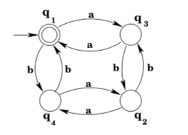
Example 3.13. Find a DFA with input alphabet \(\Sigma=\{a, b\}\) that accepts the language \(L=\left\{w \in \Sigma^{*} | n_{a}(w) \text { and } n_{b}(w) \text { are both even }\right\}\)
The characteristics that determine whether or not a string w is in L are the parity of \(n_{a}(w)\) and \(n_{b}(w)\). There are four possible combinations of “values” for these characteristics: both numbers could be even, both could be odd, the first could be odd and the second even, or the first could be even and the second odd. So we build a machine with four states \(q_{1}, q_{2}, q_{3}, q_{4}\) corresponding to the four cases. We want to set up δ so that the machine will be in state q1 exactly when it has consumed a string with an even number of a’s and an even number of b’s, in state \(q_{2}\) exactly when it has consumed a string with an odd number of a’s and an odd number of b’s, and so on.
To do this, we first make the state \(q_{1}\) into our start state, because the DFA will be in the start state after consuming the empty string ε, and ε has an even number (zero) of both a’s and b’s. Now we add transitions by reasoning about how the parity of a’s and b’s is changed by additional input. For instance, if the machine is in \(q_{1}\) (meaning an even number of a’s and an even number of b’s have been seen) and a further a is consumed, then we want the machine to move to state \(q_{3}\), since the machine has now consumed an odd number of a’s and still an even number of b’s. So we add the transition \(\delta\left(q_{1}, a\right)=q_{3}\) to the machine. Similarly, if the machine is in \(q_{2}\) (meaning an odd number of a’s and an odd number of b’s have been seen) and a further b is consumed, then we want the machine to move to state \(q_{3}\) again, since the machine has still consumed an odd number of a’s, and now an even number of b’s. So we add the transition \(\delta\left(q_{2}, b\right)=q_{3}\) to the machine. Similar reasoning produces a total of eight transitions, one for each state-input pair. Finally, we have to decide which states should be final states. The only state that corresponds to the desired criteria for the language L is \(q_{1}\), so we make \(q_{1}\) a final state. The complete machine is shown below.
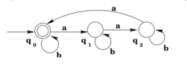
Example 3.14. Find a DFA with input alphabet Σ = {a, b} that accepts the language \(L=\left\{w \in \Sigma^{*} | n_{a}(w) \text { is divisible by } 3\right\}\).
The relevant characteristic here is of course whether or not the number of a’s in a string is divisible by 3, perhaps suggesting a two-state machine. But in fact, there is more than one way for a number to not be divisible by 3: dividing the number by 3 could produce a remainder of either 1 or 2 (a remainder of 0 corresponds to the number in fact being divisible by 3).
So we build a machine with three states \(q_{0}, q_{1}, q_{2}\), and add transitions so that the machine will be in state \(q_{0}\) exactly when the number of a’s it has consumed is evenly divisible by 3, in state \(q_{1}\) exactly when the number ofa’s it has consumed is equivalent to 1 mod 3, and similarly for \(q_{2}\). State \(q_{0}\) will be the start state, as ε has 0 a’s and 0 is divisible by 3. The completed machine is shown below. Notice that because the consumption of a b does not affect the only relevant characteristic, b’s do not cause changes of state.
Example 3.15. Find a DFA with input alphabet Σ = {a, b} that accepts the language \(L=\left\{w \in \Sigma^{*} | w \text { contains three consecutive a's }\right\}\)
Again, it is not quite so simple as making a two-state machine where the states correspond to “have seen aaa” and “have not seen aaa”. Think dynamically: as you move through the input string, how do you arrive at the goal of having seen three consecutive a’s? You might have seen two consecutive a’s and still need a third, or you might just have seen one aand be looking for two more to come immediately, or you might just have seen a b and be right back at the beginning as far as seeing 3 consecutivea’s goes. So once again there will be three states, with the “last symbol was not an a” state being the start state. The complete automaton is shown below.

Exercises
1. Give DFAs that accept the following languages over Σ = {a, b}.
a) \(L_{1}=\{x | x \text { contains the substring aba }\}\)
b) \(L_{2}=L\left(a^{*} b^{*}\right)\)
c) \(L_{3}=\left\{x | n_{a}(x)+n_{b}(x) \text { is even }\right\}\)
d) \(L_{4}=\left\{x | n_{a}(x) \text { is a multiple of } 5\right\}\)
e) \(L_{5}=\{x | x \text { does not contain the substring } a b b\}\)
f) \(L_{6}=\left\{x | x \text { has no } a^{\prime} s \text { in the even positions }\right\}\)
g) \(L_{7}=L\left(a a^{*} | a b a^{*} b^{*}\right)\)
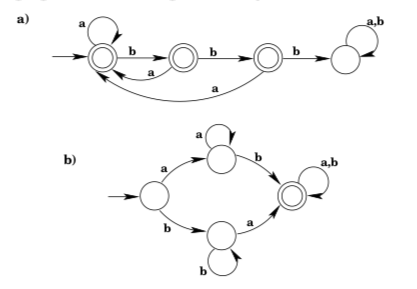
2. What languages do the following DFAs accept?
3. Let Σ = {0, 1}. Give a DFA that accepts the language
\(L=\left\{x \in \Sigma^{*} | x \text { is the binary representation of an integer divisible by } 3\right\}\)


