2.2: Elemental Signals
- Page ID
- 1600

\( \newcommand{\vecs}[1]{\overset { \scriptstyle \rightharpoonup} {\mathbf{#1}} } \)
\( \newcommand{\vecd}[1]{\overset{-\!-\!\rightharpoonup}{\vphantom{a}\smash {#1}}} \)
\( \newcommand{\dsum}{\displaystyle\sum\limits} \)
\( \newcommand{\dint}{\displaystyle\int\limits} \)
\( \newcommand{\dlim}{\displaystyle\lim\limits} \)
\( \newcommand{\id}{\mathrm{id}}\) \( \newcommand{\Span}{\mathrm{span}}\)
( \newcommand{\kernel}{\mathrm{null}\,}\) \( \newcommand{\range}{\mathrm{range}\,}\)
\( \newcommand{\RealPart}{\mathrm{Re}}\) \( \newcommand{\ImaginaryPart}{\mathrm{Im}}\)
\( \newcommand{\Argument}{\mathrm{Arg}}\) \( \newcommand{\norm}[1]{\| #1 \|}\)
\( \newcommand{\inner}[2]{\langle #1, #2 \rangle}\)
\( \newcommand{\Span}{\mathrm{span}}\)
\( \newcommand{\id}{\mathrm{id}}\)
\( \newcommand{\Span}{\mathrm{span}}\)
\( \newcommand{\kernel}{\mathrm{null}\,}\)
\( \newcommand{\range}{\mathrm{range}\,}\)
\( \newcommand{\RealPart}{\mathrm{Re}}\)
\( \newcommand{\ImaginaryPart}{\mathrm{Im}}\)
\( \newcommand{\Argument}{\mathrm{Arg}}\)
\( \newcommand{\norm}[1]{\| #1 \|}\)
\( \newcommand{\inner}[2]{\langle #1, #2 \rangle}\)
\( \newcommand{\Span}{\mathrm{span}}\) \( \newcommand{\AA}{\unicode[.8,0]{x212B}}\)
\( \newcommand{\vectorA}[1]{\vec{#1}} % arrow\)
\( \newcommand{\vectorAt}[1]{\vec{\text{#1}}} % arrow\)
\( \newcommand{\vectorB}[1]{\overset { \scriptstyle \rightharpoonup} {\mathbf{#1}} } \)
\( \newcommand{\vectorC}[1]{\textbf{#1}} \)
\( \newcommand{\vectorD}[1]{\overrightarrow{#1}} \)
\( \newcommand{\vectorDt}[1]{\overrightarrow{\text{#1}}} \)
\( \newcommand{\vectE}[1]{\overset{-\!-\!\rightharpoonup}{\vphantom{a}\smash{\mathbf {#1}}}} \)
\( \newcommand{\vecs}[1]{\overset { \scriptstyle \rightharpoonup} {\mathbf{#1}} } \)
\(\newcommand{\longvect}{\overrightarrow}\)
\( \newcommand{\vecd}[1]{\overset{-\!-\!\rightharpoonup}{\vphantom{a}\smash {#1}}} \)
\(\newcommand{\avec}{\mathbf a}\) \(\newcommand{\bvec}{\mathbf b}\) \(\newcommand{\cvec}{\mathbf c}\) \(\newcommand{\dvec}{\mathbf d}\) \(\newcommand{\dtil}{\widetilde{\mathbf d}}\) \(\newcommand{\evec}{\mathbf e}\) \(\newcommand{\fvec}{\mathbf f}\) \(\newcommand{\nvec}{\mathbf n}\) \(\newcommand{\pvec}{\mathbf p}\) \(\newcommand{\qvec}{\mathbf q}\) \(\newcommand{\svec}{\mathbf s}\) \(\newcommand{\tvec}{\mathbf t}\) \(\newcommand{\uvec}{\mathbf u}\) \(\newcommand{\vvec}{\mathbf v}\) \(\newcommand{\wvec}{\mathbf w}\) \(\newcommand{\xvec}{\mathbf x}\) \(\newcommand{\yvec}{\mathbf y}\) \(\newcommand{\zvec}{\mathbf z}\) \(\newcommand{\rvec}{\mathbf r}\) \(\newcommand{\mvec}{\mathbf m}\) \(\newcommand{\zerovec}{\mathbf 0}\) \(\newcommand{\onevec}{\mathbf 1}\) \(\newcommand{\real}{\mathbb R}\) \(\newcommand{\twovec}[2]{\left[\begin{array}{r}#1 \\ #2 \end{array}\right]}\) \(\newcommand{\ctwovec}[2]{\left[\begin{array}{c}#1 \\ #2 \end{array}\right]}\) \(\newcommand{\threevec}[3]{\left[\begin{array}{r}#1 \\ #2 \\ #3 \end{array}\right]}\) \(\newcommand{\cthreevec}[3]{\left[\begin{array}{c}#1 \\ #2 \\ #3 \end{array}\right]}\) \(\newcommand{\fourvec}[4]{\left[\begin{array}{r}#1 \\ #2 \\ #3 \\ #4 \end{array}\right]}\) \(\newcommand{\cfourvec}[4]{\left[\begin{array}{c}#1 \\ #2 \\ #3 \\ #4 \end{array}\right]}\) \(\newcommand{\fivevec}[5]{\left[\begin{array}{r}#1 \\ #2 \\ #3 \\ #4 \\ #5 \\ \end{array}\right]}\) \(\newcommand{\cfivevec}[5]{\left[\begin{array}{c}#1 \\ #2 \\ #3 \\ #4 \\ #5 \\ \end{array}\right]}\) \(\newcommand{\mattwo}[4]{\left[\begin{array}{rr}#1 \amp #2 \\ #3 \amp #4 \\ \end{array}\right]}\) \(\newcommand{\laspan}[1]{\text{Span}\{#1\}}\) \(\newcommand{\bcal}{\cal B}\) \(\newcommand{\ccal}{\cal C}\) \(\newcommand{\scal}{\cal S}\) \(\newcommand{\wcal}{\cal W}\) \(\newcommand{\ecal}{\cal E}\) \(\newcommand{\coords}[2]{\left\{#1\right\}_{#2}}\) \(\newcommand{\gray}[1]{\color{gray}{#1}}\) \(\newcommand{\lgray}[1]{\color{lightgray}{#1}}\) \(\newcommand{\rank}{\operatorname{rank}}\) \(\newcommand{\row}{\text{Row}}\) \(\newcommand{\col}{\text{Col}}\) \(\renewcommand{\row}{\text{Row}}\) \(\newcommand{\nul}{\text{Nul}}\) \(\newcommand{\var}{\text{Var}}\) \(\newcommand{\corr}{\text{corr}}\) \(\newcommand{\len}[1]{\left|#1\right|}\) \(\newcommand{\bbar}{\overline{\bvec}}\) \(\newcommand{\bhat}{\widehat{\bvec}}\) \(\newcommand{\bperp}{\bvec^\perp}\) \(\newcommand{\xhat}{\widehat{\xvec}}\) \(\newcommand{\vhat}{\widehat{\vvec}}\) \(\newcommand{\uhat}{\widehat{\uvec}}\) \(\newcommand{\what}{\widehat{\wvec}}\) \(\newcommand{\Sighat}{\widehat{\Sigma}}\) \(\newcommand{\lt}{<}\) \(\newcommand{\gt}{>}\) \(\newcommand{\amp}{&}\) \(\definecolor{fillinmathshade}{gray}{0.9}\)- Complex signals can be built from elemental signals, including the complex exponential, unit step, pulse, etc.
- Learning about elemental signals.
Elemental signals are the building blocks with which we build complicated signals. By definition, elemental signals have a simple structure. Exactly what we mean by the "structure of a signal" will unfold in this section of the course. Signals are nothing more than functions defined with respect to some independent variable, which we take to be time for the most part. Very interesting signals are not functions solely of time; one great example of which is an image. For it, the independent variables are x and y (two-dimensional space). Video signals are functions of three variables: two spatial dimensions and time. Fortunately, most of the ideas underlying modern signal theory can be exemplified with one-dimensional signals.
Sinusoids
Perhaps the most common real-valued signal is the sinusoid.
\[s(t) = A\cos (2\pi f_{0}t+\varphi ) \nonumber \]
For this signal, is its amplitude, its frequency, and its phase.
Complex Exponentials
The most important signal is complex-valued, the complex exponential.
\[s(t) = Ae^{i(2\pi f_{0}t+\varphi )}\\ s(t) = Ae^{i\varphi }e^{i2\pi f_{0}t} \nonumber \]
Here,
\[Ae^{i\varphi } \: is\: the\: signal's\: \textbf{complex amplitude} \nonumber \]
Considering the complex amplitude as a complex number in polar form, its magnitude is the amplitude A and its angle the signal phase. The complex amplitude is also known as a phasor. The complex exponential cannot be further decomposed into more elemental signals, and is the most important signal in electrical engineering! Mathematical manipulations at first appear to be more difficult because complex-valued numbers are introduced. In fact, early in the twentieth century, mathematicians thought engineers would not be sufficiently sophisticated to handle complex exponentials even though they greatly simplified solving circuit problems. Steinmetz introduced complex exponentials to electrical engineering, and demonstrated that "mere" engineers could use them to good effect and even obtain right answers! See Complex Numbers for a review of complex numbers and complex arithmetic.
The complex exponential defines the notion of frequency: it is the only signal that contains only one frequency component. The sinusoid consists of two frequency components: one at the frequency f0 and the other at -f0.
This decomposition of the sinusoid can be traced to Euler's relation.
\[\cos (2\pi ft) = \frac{e^{i2\pi ft}+e^{-(i2\pi ft)}}{2}\\ \sin (2\pi ft) = \frac{e^{i2\pi ft}-e^{-(i2\pi ft)}}{2i}\\ e^{i2\pi ft} = cos (2\pi ft)+i\: sin (2\pi ft) \nonumber \]
The complex exponential signal can thus be written in terms of its real and imaginary parts using Euler's relation. Thus, sinusoidal signals can be expressed as either the real or the imaginary part of a complex exponential signal, the choice depending on whether cosine or sine phase is needed, or as the sum of two complex exponentials. These two decompositions are mathematically equivalent to each other.
\[A\cos (2\pi ft+\varphi ) = \Re (Ae^{i\varphi }e^{i2\pi ft})\\ A\sin (2\pi ft+\varphi ) = \Im (Ae^{i\varphi }e^{i2\pi ft}) \nonumber \]
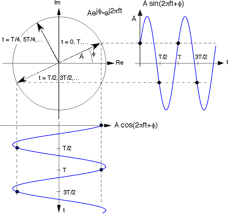
Using the complex plane, we can envision the complex exponential's temporal variations as seen in the above figure. The magnitude of the complex exponential is A and the initial value of the complex exponential at t = 0 has an angle of φ. As time increases, the locus of points traced by the complex exponential is a circle (it has constant magnitude of A). The number of times per second we go around the circle equals the frequency f. The time taken for the complex exponential to go around the circle once is known as its period T and equals 1/f. The projections onto the real and imaginary axes of the rotating vector representing the complex exponential signal are the cosine and sine signal of Euler's relation as stated above.
Real Exponentials
As opposed to complex exponentials which oscillate, real exponentials decay.
\[s(t) = e^{-\frac{t}{\tau }} \nonumber \]
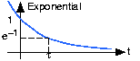
The quantity τ is known as the exponential's time constant, and corresponds to the time required for the exponential to decrease by a factor of 1/e, which approximately equals 0.368. A decaying complex exponential is the product of a real and a complex exponential.
\[s(t) = Ae^{i\varphi }e^{-\frac{t}{\tau }}e^{i2\pi ft}\\ s(t) = Ae^{i\varphi }e^{\left ( -\frac{t}\tau +i2\pi f \right )t} \nonumber \]
In the complex plane, this signal corresponds to an exponential spiral. For such signals, we can define complex frequency as the quantity multiplying t.
Unit Step
The unit step function is denoted by u(t), and is defined to be
\[u(t) = 0\, \, if \,\, t< 0\\ u(t) = 1\, \: if \, \, t> 0 \nonumber \]
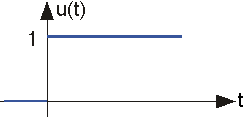
Figure 2.2.3 Unit Step
This signal is discontinuous at the origin. Its value at the origin need not be defined, and doesn't matter in signal theory.
This kind of signal is used to describe signals that "turn on" suddenly. For example, to mathematically represent turning on an oscillator, we can write it as the product of a sinusoid and a step:
\[s(t) = A\sin (2\pi ft)u(t) \nonumber \]
Pulse
The unit pulse describes turning a unit-amplitude signal on for a duration of Δ seconds, then turning it off.
\[p\Delta (t) = 0\; if\; t< 0\\ p\Delta (t) = 1\; if\; 0< t< \Delta \\ p\Delta (t) = 0\; if\; t> \Delta \nonumber \]
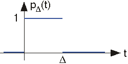
We will find that this is the second most important signal in communications.
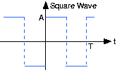
Square Wave
The square wave sq(t) is a periodic signal like the sinusoid. It too has an amplitude and a period, which must be specified to characterize the signal. We find subsequently that the sine wave is a simpler signal than the square wave.