5.11: Ohmic Conduction and Convection in Steady State- D-C Interactions
- Page ID
- 51484
\( \newcommand{\vecs}[1]{\overset { \scriptstyle \rightharpoonup} {\mathbf{#1}} } \)
\( \newcommand{\vecd}[1]{\overset{-\!-\!\rightharpoonup}{\vphantom{a}\smash {#1}}} \)
\( \newcommand{\dsum}{\displaystyle\sum\limits} \)
\( \newcommand{\dint}{\displaystyle\int\limits} \)
\( \newcommand{\dlim}{\displaystyle\lim\limits} \)
\( \newcommand{\id}{\mathrm{id}}\) \( \newcommand{\Span}{\mathrm{span}}\)
( \newcommand{\kernel}{\mathrm{null}\,}\) \( \newcommand{\range}{\mathrm{range}\,}\)
\( \newcommand{\RealPart}{\mathrm{Re}}\) \( \newcommand{\ImaginaryPart}{\mathrm{Im}}\)
\( \newcommand{\Argument}{\mathrm{Arg}}\) \( \newcommand{\norm}[1]{\| #1 \|}\)
\( \newcommand{\inner}[2]{\langle #1, #2 \rangle}\)
\( \newcommand{\Span}{\mathrm{span}}\)
\( \newcommand{\id}{\mathrm{id}}\)
\( \newcommand{\Span}{\mathrm{span}}\)
\( \newcommand{\kernel}{\mathrm{null}\,}\)
\( \newcommand{\range}{\mathrm{range}\,}\)
\( \newcommand{\RealPart}{\mathrm{Re}}\)
\( \newcommand{\ImaginaryPart}{\mathrm{Im}}\)
\( \newcommand{\Argument}{\mathrm{Arg}}\)
\( \newcommand{\norm}[1]{\| #1 \|}\)
\( \newcommand{\inner}[2]{\langle #1, #2 \rangle}\)
\( \newcommand{\Span}{\mathrm{span}}\) \( \newcommand{\AA}{\unicode[.8,0]{x212B}}\)
\( \newcommand{\vectorA}[1]{\vec{#1}} % arrow\)
\( \newcommand{\vectorAt}[1]{\vec{\text{#1}}} % arrow\)
\( \newcommand{\vectorB}[1]{\overset { \scriptstyle \rightharpoonup} {\mathbf{#1}} } \)
\( \newcommand{\vectorC}[1]{\textbf{#1}} \)
\( \newcommand{\vectorD}[1]{\overrightarrow{#1}} \)
\( \newcommand{\vectorDt}[1]{\overrightarrow{\text{#1}}} \)
\( \newcommand{\vectE}[1]{\overset{-\!-\!\rightharpoonup}{\vphantom{a}\smash{\mathbf {#1}}}} \)
\( \newcommand{\vecs}[1]{\overset { \scriptstyle \rightharpoonup} {\mathbf{#1}} } \)
\(\newcommand{\longvect}{\overrightarrow}\)
\( \newcommand{\vecd}[1]{\overset{-\!-\!\rightharpoonup}{\vphantom{a}\smash {#1}}} \)
\(\newcommand{\avec}{\mathbf a}\) \(\newcommand{\bvec}{\mathbf b}\) \(\newcommand{\cvec}{\mathbf c}\) \(\newcommand{\dvec}{\mathbf d}\) \(\newcommand{\dtil}{\widetilde{\mathbf d}}\) \(\newcommand{\evec}{\mathbf e}\) \(\newcommand{\fvec}{\mathbf f}\) \(\newcommand{\nvec}{\mathbf n}\) \(\newcommand{\pvec}{\mathbf p}\) \(\newcommand{\qvec}{\mathbf q}\) \(\newcommand{\svec}{\mathbf s}\) \(\newcommand{\tvec}{\mathbf t}\) \(\newcommand{\uvec}{\mathbf u}\) \(\newcommand{\vvec}{\mathbf v}\) \(\newcommand{\wvec}{\mathbf w}\) \(\newcommand{\xvec}{\mathbf x}\) \(\newcommand{\yvec}{\mathbf y}\) \(\newcommand{\zvec}{\mathbf z}\) \(\newcommand{\rvec}{\mathbf r}\) \(\newcommand{\mvec}{\mathbf m}\) \(\newcommand{\zerovec}{\mathbf 0}\) \(\newcommand{\onevec}{\mathbf 1}\) \(\newcommand{\real}{\mathbb R}\) \(\newcommand{\twovec}[2]{\left[\begin{array}{r}#1 \\ #2 \end{array}\right]}\) \(\newcommand{\ctwovec}[2]{\left[\begin{array}{c}#1 \\ #2 \end{array}\right]}\) \(\newcommand{\threevec}[3]{\left[\begin{array}{r}#1 \\ #2 \\ #3 \end{array}\right]}\) \(\newcommand{\cthreevec}[3]{\left[\begin{array}{c}#1 \\ #2 \\ #3 \end{array}\right]}\) \(\newcommand{\fourvec}[4]{\left[\begin{array}{r}#1 \\ #2 \\ #3 \\ #4 \end{array}\right]}\) \(\newcommand{\cfourvec}[4]{\left[\begin{array}{c}#1 \\ #2 \\ #3 \\ #4 \end{array}\right]}\) \(\newcommand{\fivevec}[5]{\left[\begin{array}{r}#1 \\ #2 \\ #3 \\ #4 \\ #5 \\ \end{array}\right]}\) \(\newcommand{\cfivevec}[5]{\left[\begin{array}{c}#1 \\ #2 \\ #3 \\ #4 \\ #5 \\ \end{array}\right]}\) \(\newcommand{\mattwo}[4]{\left[\begin{array}{rr}#1 \amp #2 \\ #3 \amp #4 \\ \end{array}\right]}\) \(\newcommand{\laspan}[1]{\text{Span}\{#1\}}\) \(\newcommand{\bcal}{\cal B}\) \(\newcommand{\ccal}{\cal C}\) \(\newcommand{\scal}{\cal S}\) \(\newcommand{\wcal}{\cal W}\) \(\newcommand{\ecal}{\cal E}\) \(\newcommand{\coords}[2]{\left\{#1\right\}_{#2}}\) \(\newcommand{\gray}[1]{\color{gray}{#1}}\) \(\newcommand{\lgray}[1]{\color{lightgray}{#1}}\) \(\newcommand{\rank}{\operatorname{rank}}\) \(\newcommand{\row}{\text{Row}}\) \(\newcommand{\col}{\text{Col}}\) \(\renewcommand{\row}{\text{Row}}\) \(\newcommand{\nul}{\text{Nul}}\) \(\newcommand{\var}{\text{Var}}\) \(\newcommand{\corr}{\text{corr}}\) \(\newcommand{\len}[1]{\left|#1\right|}\) \(\newcommand{\bbar}{\overline{\bvec}}\) \(\newcommand{\bhat}{\widehat{\bvec}}\) \(\newcommand{\bperp}{\bvec^\perp}\) \(\newcommand{\xhat}{\widehat{\xvec}}\) \(\newcommand{\vhat}{\widehat{\vvec}}\) \(\newcommand{\uhat}{\widehat{\uvec}}\) \(\newcommand{\what}{\widehat{\wvec}}\) \(\newcommand{\Sighat}{\widehat{\Sigma}}\) \(\newcommand{\lt}{<}\) \(\newcommand{\gt}{>}\) \(\newcommand{\amp}{&}\) \(\definecolor{fillinmathshade}{gray}{0.9}\)The one-dimensional configuration of Fig. 5.7.1 is revisited in this section using an ohmic rather than a unipolar model. This gives the opportunity to exemplify the role of the electric field and boundary conditions while making a contrast between the ohmic model, introduced in Sec. 5.10 and the unipolar model of Sec. 5.7. As in Sec. 5.7, the model is used to demonstrate a type of "d-c" pump or generator exploiting longitudinal stresses. Again, screen electrodes are used to charge a uniform z-directed flow: \(\overrightarrow{v} = U \overrightarrow{i}_z\).
Because the fluid has uniform properties, the steady one-dimensional form of Eq. 5.10.6 is
\[ \frac{d \rho_f}{dz} + \frac{\sigma}{U \varepsilon} \rho_f = 0 \label{1} \]
and it follows directly that the space-charge distribution is exponential:
\[ \rho_f = \rho_o e^{-z/R_e l} ; \, R_e \equiv \frac{\varepsilon v}{ \sigma l} \label{2} \]
The electric Reynolds number \(R_e\) is introduced at this point because it reflects such attributes of the flow as the efficiency of energy conversion.
Conservation of charge requires that in the steady state \(\overrightarrow{J}_f = J \overrightarrow{i}_z\) is a constant: the total current \(I\) divided by the area \(A\). Thus the constitutive law, Eq. 5.10.2, can be solved for \(\overrightarrow{E} = E(z) \overrightarrow{i}_z\) with \(\rho_f\) substituted from Eq. \ref{2}:
\[ E = \frac{i}{\sigma A} - \frac{\rho_o U}{\sigma} e^{-z/ R_e l} \label{3} \]
In turn, the terminal potential is determined,
\[ v = -\int_0^l E dz = - \frac{il}{\sigma A} + \frac{\rho_o l U}{\sigma} R_e ( 1 - e^{-1/R_e}) \label{4} \]
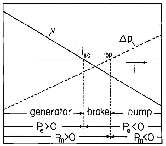
This is the electrical terminal relation for the interaction: a "volt-ampere" characteristic sketched in Fig. 5.11.1.
The electrical force on the charged particles is fully transmitted to the vehicle fluid, and hence the pressure rise between inlet and outlet is simply the difference in electric stresses at \(z = l\) and \(z = 0\), evaluated using Eq. \ref{3}:
\[ \Delta p = P_o - P_i = \frac{1}{2} \varepsilon [E^2 (l) - E^2(0)] = \frac{1}{2} \varepsilon [ (\frac{i}{\sigma A} - \frac{\rho_o U}{\sigma} e^{-1/R_e})^2 - (\frac{i}{\sigma A} - \frac{\rho_o U}{\sigma})^2] \label{5} \]
This mechanical "terminal relation" has a dependence on the terminal current \(i\) summarized by Fig. 5.11.1. Observe that \(i_{sc} < i_{bp}\), where the short-circuit and zero pressure-rise currents follow from setting Eqs. \ref{4} and \ref{5} to zero:
\[ I_{sc} = A \rho_o U R_e ( 1- e^{-1/R_e}) \label{6} \]
\[ I_{bp} = A \rho_o U (1+ e^{-1/R_e})/2 \label{7} \]
Three energy conversion regimes are defined by recognizing that the electrical power out is \(P_e = VI\), while the mechanical power in is \(P_m = -\Delta p U A\). Each of these quantities must be positive to give a generator function. Similarly, if both \(P_e\) and \(P_m\) are negative, energy is converted from electrical to mechanical form and the device is a pump. There is a midregion, which tends to vanish as \(R_e\) is increased, wherein both electrical and mechanical energy are absorbed. This region gives a braking effect at the expense of electrical energy. These three regimes are summarized by Fig. 5.11.1.
The Generator Interaction
A primary limitation on electrohydrodynamic energy conversion devices is the relatively small electric pressure that can be obtained without incurring electrical breakdown. Difficulties in making an efficient converter are amplified by the extremely small fraction of the available mechanical energy that is altered by the electric coupling. It is clear from Eq. \ref{5} that any electric stress at the outlet detracts from the total pressure change. To take the greatest advantage of the available electric stress, \(E(l)\) should be adjusted to vanish. This can be done, according to Eq. \ref{3}, by operating with the space-charge density
\[ \rho_o v = \frac{I}{A} e^{1/R_e} \label{8} \]
It follows from Eq. \ref{4} that (use upper sign):
\[ P_e = - \frac{I^2 l}{ \sigma A} [ 1 \pm R_e (1 - e^{\pm 1/R_e})] \label{9} \]
while Eq. \ref{5} shows that (upper sign)
\[ P_m = \pm \frac{U A \varepsilon}{2} (\frac{i}{\sigma A})^2 (1 - e^{\pm 1 /R_e})^2 \label{10} \]
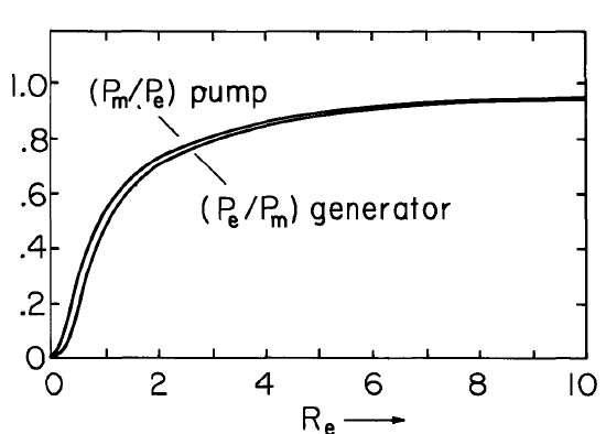
The efficiency of energy conversion.from mechanical to electrical form is then only a function of the electric Reynolds number (upper sign)
\[ P_e/P_m = 2 \dfrac{\pm R_e (e^{\pm 1 /R_e} - 1) - 1}{\pm R_e (1- e^{\pm 1/R_e})^2} \label{11} \]
Of course, the conversion becomes perfectly efficient as \(R_e \rightarrow \infty\). The detailed dependence is shown in Fig. 5.11.2.
The Pump Interaction
If it is a pumping function that is desired, Eq. \ref{5} makes it clear that the space charge should be adjusted so that \(E(0) = 0\), and it follows from Eq. \ref{3} that
\[ \frac{i}{A} = \rho_o v \label{12} \]
The electrical and mechanical powers are now given by Eqs. \ref{9} and \ref{10} using the lower signs. In turn, the efficiency of electrical to mechanical conversion is the reciprocal of Eq. \ref{11}, using the lower signs.This pumping efficiency is summarized also in Fig. 5.11.2.