6.1: Faraday's Law of Induction

6-1-1 The Electromotive Force (EMF)

Faraday's original experiments consisted of a conducting loop through which he could impose a dc current via a switch. Another short circuited loop with no source attached was nearby, as shown in Figure 6-1. When a dc current flowed in loop 1, no current flowed in loop 2. However, when the voltage was first applied to loop 1 by closing the switch, a transient current flowed in the opposite direction in loop 2.

Figure 6-1 Faraday's experiments showed that a time varying magnetic flux through a closed conducting loop induced a current in the direction so as to keep the flux through the loop constant.

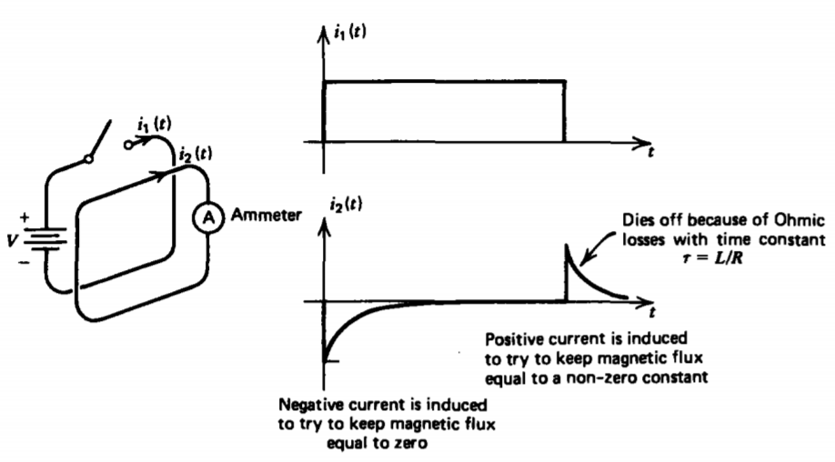
When the switch was later opened, another transient current flowed in loop 2, this time in the same direction as the original current in loop 1. Currents are induced in loop 2 whenever a time varying magnetic flux due to loop 1 passes through it.

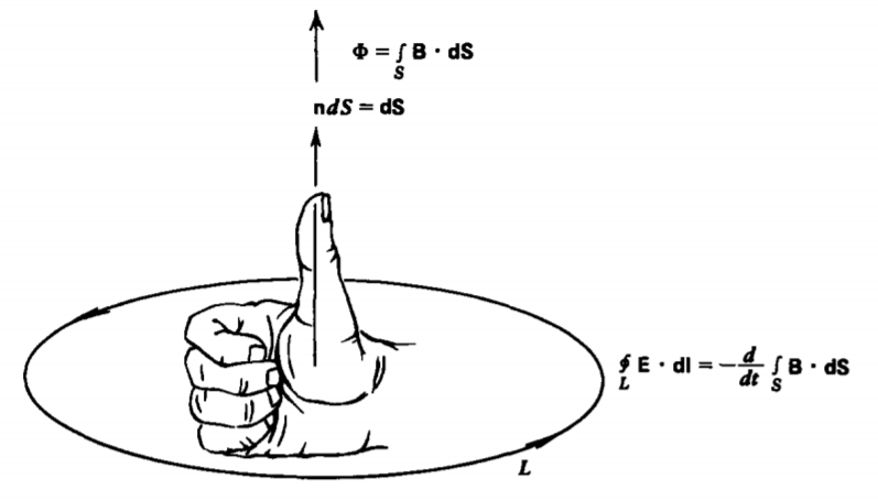
In general, a time varying magnetic flux can pass through a circuit due to its own or nearby time varying current or by the motion of the circuit through a magnetic field. For any loop, as in Figure 6-2, Faraday's law is

\[\textrm{EMF} = \oint_{L} \textbf{E} \cdot \textbf{dl} = - \frac{d \Phi}{dt} = - \frac{d}{dt} \int_{S} \textbf{B} \cdot \textbf{dS} \]

where EMF is the electromotive force defined as the line integral of the electric field. The minus sign is introduced on the right-hand side of (1) as we take the convention that positive flux flows in the direction perpendicular to the direction of the contour by the right-hand rule.

6-1-2 Lenz's Law

The direction of induced currents is always such as to oppose any changes in the magnetic flux already present. Thus in Faraday's experiment, illustrated in Figure 6-1, when the switch in loop 1 is first closed there is no magnetic flux in loop 2 so that the induced current flows in the opposite direction with its self-magnetic field opposite to the imposed field. The induced current tries to keep a zero flux through

Figure 6-2 Faraday's law states that the line integral of the electric field around a closed loop equals the time rate of change of magnetic flux through the loop. The positive convention for flux is determined by the right-hand rule of curling the fingers on the right hand in the direction of traversal around the loop. The thumb then points in the direction of positive magnetic flux.

loop 2. If the loop is perfectly conducting, the induced current flows as long as current flows in loop 1, with zero net flux through the loop. However, in a real loop, resistive losses cause the current to exponentially decay with an L/R time constant, where L is the self-inductance of the loop and R is its resistance. Thus, in the dc steady state the induced current has decayed to zero so that a constant magnetic flux passes through loop 2 due to the current in loop 1.

When the switch is later opened so that the current in loop 1 goes to zero, the second loop tries to maintain the constant flux already present by inducing a current flow in the same direction as the original current in loop 1. Ohmic losses again make this induced current die off with time.

If a circuit or any part of a circuit is made to move through a magnetic field, currents will be induced in the direction such as to try to keep the magnetic flux through the loop constant. The force on the moving current will always be opposite to the direction of motion.

Lenz's law is clearly demonstrated by the experiments shown in Figure 6-3. When a conducting ax is moved into a magnetic field, eddy currents are induced in the direction where their self-flux is opposite to the applied magnetic field. The Lorentz force is then in the direction opposite to the motion of the ax. This force decreases with time as the currents decay with time due to Ohmic dissipation. If the ax was slotted, effectively creating a very high resistance to the eddy currents, the reaction force becomes very small as the induced current is small.

Figure 6-3 Lenz's law. (a) Currents induced in a conductor moving into a magnetic field exert a force opposite to the motion. The induced currents can be made small by slotting the ax. (b) A conducting ring on top of a coll is flipped off when a current is suddenly applied, as the induced currents try to keep a zero flux through the ring.

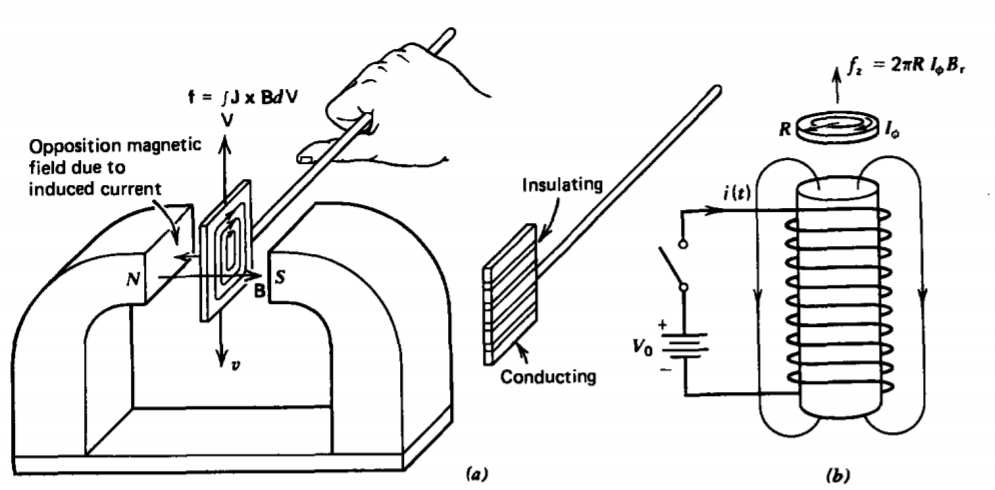
\[ \mathrm{f}=2 \pi R I \times B=2 \pi R I_\phi B_{\mathrm{r}} \mathbf{i}_z \]

which flips the ring off the coil. If the ring is cut radially so that no circulating current can flow, the force is zero and the ring does not move

(a) Short Circuited Loop

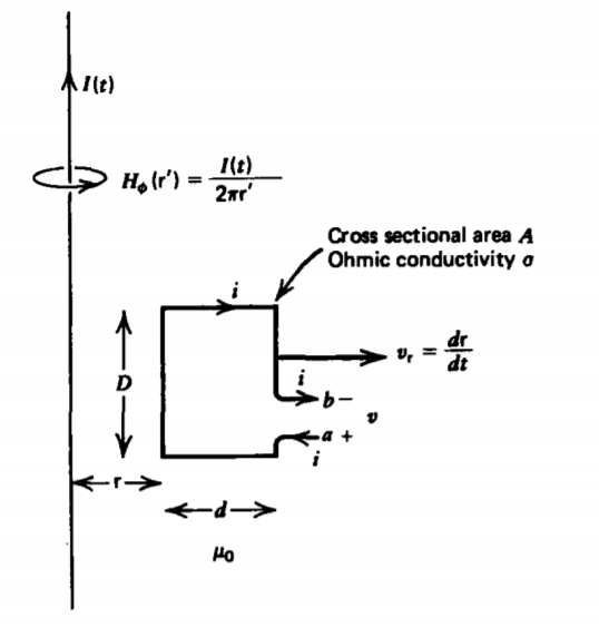
To be quantitative, consider the infinitely long time varying line current I(t) in Figure 6-4, a distance r from a rectangular loop of wire with Ohmic conductivity \(\sigma\), cross-sectional area A, and total length \(l = 2(D + d)\). The magnetic flux through the loop due to I(t) is

\[\Phi_{m} = \int_{z= -D/2}^{D/2} \int_{\textrm{r}}^{\textrm{r} + d} \mu_{0} H_{\phi}(\textrm{r}') d \textrm{r}' dz \\ = \frac{\mu_{0}ID}{2 \pi} \int_{\textrm{r}}^{\textrm{r} + d} \frac{d \textrm{r}'}{\textrm{r}'} = \frac{\mu_{0} ID}{2 \pi} \ln \frac{\textrm{r} + d}{\textrm{r}} \]

Figure 6-4 A rectangular loop near a time varying line current. When the terminals are short circuited the electromotive force induces a current due to the time varying mutual flux and/or because of the motion of the circuit through the imposed nonuniform magnetic field of the line current. If the loop terminals are open circuited there is no induced current but a voltage develops.

The mutual inductance M is defined as the flux to current ratio where the flux through the loop is due to an external current. Then (3) becomes

\[\Phi_{m} = M(\textrm{r})I, \: \: \: \: M(\textrm{r}) = \frac{\mu_{0}D}{2 \pi} \ln \frac{\textrm{r} + d}{\textrm{r}} \]

When the loop is short circuited (\(v\) = 0), the induced Ohmic current \(i\) gives rise to an electric field [\(E = J/\sigma = i/ (A \sigma)\)] so that Faraday's law applied to a contour within the wire yields an electromotive force just equal to the Ohmic voltage drop:

\[\oint_{L} \textbf{E} \cdot \textbf{dl} = \frac{il}{\sigma A} = iR = - \frac{d \Phi}{dt} \]

where \(R = L/(\sigma A)\) is the resistance, of the loop. By convention, the current is taken as positive in the direction of the line integral.

The flux in (5) has contributions both from the imposed current as given in (3) and from the induced current proportional to the loop's self-inductance L, which for example is given in Section 5-4-3c for a square loop (D = d):

\[\Phi = M(\textrm{r}) I + Li \]

If the loop is also moving radially outward with velocity \(v_{\textrm{r}} = d \textrm{r} /dt\), the electromotively induced Ohmic voltage is

\[-iR = \frac{d \Phi}{dt} \\ = M(\textrm{r}) \frac{dI}{dt} + I \frac{dM(\textrm{r})}{dt} + L \frac{di}{dt} \\ = M(\textrm{r}) \frac{dI}{dt} + I \frac{dM}{d \textrm{r}} \frac{d \textrm{r}}{dt} + L \frac{di}{dt} \]

where L is not a function of the loop's radial position.

If the loop is stationary, only the first and third terms on the right-hand side contribute. They are nonzero only if the currents change with time. The second term is due to the motion and it has a contribution even for dc currents.

Turn-on Transient. If the loop is stationary (\(d \textrm{r}/dt = 0\)) at r = r₀, (7) reduces to

\[L \frac{di}{dt} + iR = - M(\textrm{r}_{0}) \frac{dI}{dt} \]

If the applied current I is a dc step turned on at t =0, the solution to (8) is

\[i(t) = 0 \frac{M(\textrm{r}_{0})I}{L} e^{-(R/L)t}, \: \: \: t > 0 \]

where the impulse term on the right-hand side of (8) imposes the initial condition \(i(t = 0) = -M(\textrm{r}_{0})I/L\). The current is negative, as Lenz's law requires the self-flux to oppose the applied flux.

Turn-off Transient. If after a long time T the current I is instantaneously turned off, the solution is

\[i(t) = \frac{M(\textrm{r}_{0})I}{L} e^{-(R/L)(t-T)}, \: \: \: t > T \]

where now the step decrease in current I at t = T reverses the direction of the initial current.

Motion with a dc Current. With a dc current, the first term on the right-hand side in (7) is zero yielding

\[L \frac{di}{dt} + iR = \frac{\mu_{0}IDd}{2 \pi \textrm{r}(\textrm{r} + d)} \frac{d \textrm{r}}{dt} \]

To continue, we must specify the motion so that we know how r changes with time. Let's consider the simplest case when the loop has no resistance (R = 0). Then (11) can be directly integrated a

\[Li = - \frac{\mu_{0}ID}{2 \pi} \ln \frac{1 + d/ \textrm{r}}{1 + d/ \textrm{r}_{0}} \]

where we specify that the current is zero when r =ro. This solution for a lossless loop only requires that the total flux of (6) remain constant. The current is positive when r> r₀ as the self-flux must aid the decreasing imposed flux. The current is similarly negative when r < r₀ as the self-flux must cancel the increasing imposed flux.

The force on the loop for all these cases is only due to the force on the z-directed current legs at r and r+d:

\[f_{\textrm{r}} = \frac{\mu_{0}DiI}{2 \pi} \bigg( \frac{1}{\textrm{r} + d} - \frac{1}{\textrm{r}}\bigg) \\ = - \frac{\mu_{0}DiId}{2 \pi \textrm{r}(\textrm{r} + d)} \]

being attractive if iI > 0 and repulsive if iI <0.

(b) Open Circuited Loop

If the loop is open circuited, no induced current can flow and thus the electric field within the wire is zero (\(\textbf{J} = \sigma \textbf{E} = 0\)). The electromotive force then only has a contribution from the gap between terminals equal to the negative of the voltage:

\[\oint_{L} \textbf{E} \cdot \textbf{dl} = \int_{b}^{a} \textbf{E} \cdot \textbf{dl} = - v = - \frac{d \Phi}{dt} \Rightarrow v = \frac{d \Phi}{dt} \]

Note in Figure 6-4 that our convention is such that the current i is always defined positive flowing out of the positive voltage terminal into the loop. The flux \(\Phi\) in (14) is now only due to the mutual flux given by (3), as with i =0 there is no self-flux. The voltage on the moving open circuited loop is then

\[v = M (\textrm{r}) \frac{dI}{dt} + I \frac{dM}{d \textrm{r}} \frac{d \textrm{r}}{dt} \]

(c) Reaction Force

The magnetic force on a short circuited moving loop is always in the direction opposite to its motion. Consider the short circuited loop in Figure 6-5, where one side of the loop moves with velocity \(v_{x}\). With a uniform magnetic field applied normal to the loop pointing out of the page, an expansion of the loop tends to link more magnetic flux requiring the induced current to flow clockwise so that its self-flux is in the direction given by the right-hand rule, opposite to the applied field. From (1) we have

\[\oint_{L} \textbf{E} \cdot \textbf{dl} = \frac{il}{\sigma A} = iR = - \frac{d \Phi}{dt} = B_{0}D \frac{dx}{dt} = B_{0}Dv_{x} \]

where \(l = 2 (D + x)\) also changes with time. The current is then

\[i = \dfrac{B_{0}Dv_{x}}{R} \]

Figure 6-5 If a conductor moves perpendicular to a magnetic field a current is induced in the direction to cause the Lorentz force to be opposite to the motion. The total flux through the closed loop, due to both the imposed field and the self-field generated by the induced current, tries to remain constant.

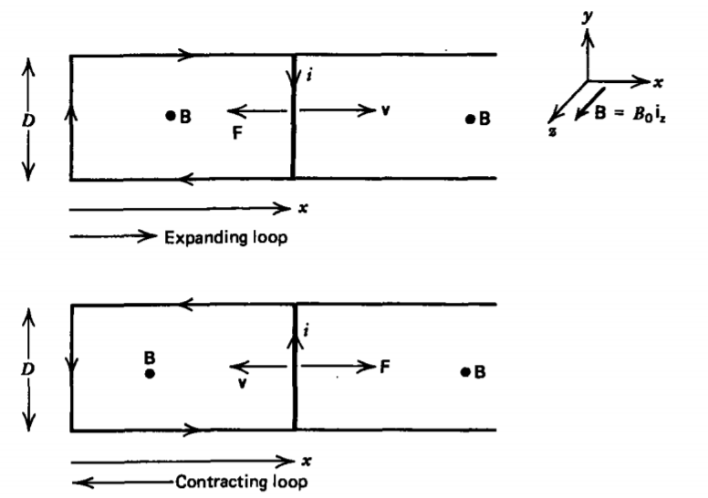
where we neglected the self-flux generated by \(i\), assuming it to be much smaller than the applied flux due to \(B_{0}\). Note also that the applied flux is negative, as the right-hand rule applied to the direction of the current defines positive flux into the page, while the applied flux points outwards.

The force on the moving side is then to the left,

\[\textbf{f} = -iD \textbf{i}_{y} \times B_{0} \textbf{i}_{z} = iD B_{0} \textbf{i}_{x} = - \frac{B_{0}^{2}D^{2}v_{x}}{R} \textbf{i}_{x} \]

opposite to the velocity.

However if the side moves to the left (\(v_{x}\) <0), decreasing the loop's area thereby linking less flux, the current reverses direction as does the force.

6-1-3 Laminations

The induced eddy currents in Ohmic conductors results in Ohmic heating. This is useful in induction furnaces that melt metals, but is undesired in many iron core devices. To reduce this power loss, the cores are often sliced into many thin sheets electrically insulated from each other by thin oxide coatings. The current flow is then confined to lie within a thin sheet and cannot cross over between sheets. The insulating laminations serve the same purpose as the cuts in the slotted ax in Figure 6-3a.

The rectangular conductor in Figure 6-6a has a time varying magnetic field B(t) passing through it. We approximate the current path as following the rectangular shape so that

Figure 6-6 (a) A time varying magnetic field through a conductor induces eddy currents that cause Ohmic heating. (b) If the conductor is laminated so that the induced currents are confined to thin strips, the dissipated power decreases.

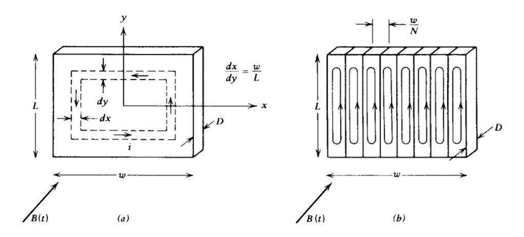
the flux through the loop of incremental width dx and dy of area 4xy is

\[\Phi = - 4 xy B (t) \]

where we neglect the reaction field of the induced current assuming it to be much smaller than the imposed field. The minus sign arises because, by the right-hand rule illustrated in Figure 6-2, positive flux flows in the direction opposite to B(t). The resistance of the loop is

\[R_{x} = \frac{4}{\sigma D} \bigg( \frac{y}{dx} + \frac{x}{dy} \bigg) = \frac{4}{\sigma D} \frac{L}{w} \frac{x}{dx} \bigg[ 1 + \bigg( \frac{w}{L} \bigg)^{2} \bigg] \]

The electromotive force around the loop then just results in an Ohmic current:

\[\oint_{L} \textbf{E} \cdot \textbf{dl} = i R_{x} = \frac{-d \Phi}{dt} = 4xy \frac{dB}{dt} = \frac{4L}{w} x^{2} \frac{dB}{dt} \]

with dissipated power

\[dp = i^{2} R_{x} = \frac{4 Dx^{3} \sigma L (dB/dt)^{2}dx}{w[1 + (w/L)^{2}]} \]

The total power dissipated over the whole sheet is then found by adding the powers dissipated in each incremental loop:

\[P = \int_{0}^{w/2} dp \\ = \frac{4D (dB/dt)^{2}\sigma L}{wp1 + (w/L)^{2}]} \int_{0}^{w/2} x^{3}dx \\ = \frac{LDw^{3} \sigma (dB/dt)^{2}}{16[1 _ w/L)^{2}]} \]

If the sheet is laminated into N smaller ones, as in Figure 6-6b, each section has the same solution as (23) if we replace w by wIN. The total power dissipated is then N times the power dissipated in a single section:

\[P = \frac{LD (w/N)^{3} \sigma (dB/dt)^{2}N}{16[1 + (w/NL)^{2}]} = \frac{\sigma L D w^{3} (dB/dt)^{2}}{16 N^{2}[1 + (w/NL)^{2}]} \]

As N becomes large so that \(w/NL <<1\), the dissipated power decreases as 1/N ².

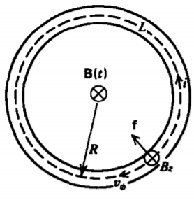
6-1-4 Betatron

The cyclotron, discussed in Section 5-1-4, is not used to accelerate electrons because their small mass allows them to reach relativistic speeds, thereby increasing their mass and decreasing their angular speed. This puts them out of phase with the applied voltage. The betatron in Figure 6-7 uses the transformer principle where the electrons circulating about the evacuated toroid act like a secondary winding. The imposed time varying magnetic flux generates an electric field that accelerates the electrons.

Faraday's law applied to a contour following the charge's trajectory at radius R yields

\[\oint_{L} \textbf{E} \cdot \textbf{dl} = E_{\phi} 2 \piR = - \frac{d \Phi}{dt} \]

which accelerates the electrons as

\[m \frac{dv_{\phi}}{dt} = - eE_{\phi} = \frac{e}{2 \pi R} \frac{d \Phi}{dt} \Rightarrow v_{\phi} = \frac{e}{2 \pi m R} \Phi \]

The electrons move in the direction so that their selfmagnetic flux is opposite to the applied flux. The resulting Lorentz force is radially inward. A stable orbit of constant radius R is achieved if this force balances the centrifugal force:

\[m \frac{dv_{r}}{dt} = \frac{mv^{2}_{\phi}}{R} - ev_{\phi}B_{z}(R) = 0 \]

which from (26) requires the flux and magnetic field to be related as

\[\Phi = 2 \pi R^{2} B_{z} (R) \]

This condition cannot be met by a uniform field (as then \(\Phi = \pi R^{2} B_{z}\)) so in practice the imposed field is made to approximately vary with radial position as

\[B_{z}(r) = B_{0} \bigg( \frac{R}{r} \bigg) \Rightarrow \Phi = 2 \pi \int_{r = 0}^{R} B_{z} (r)r \: dr = 2 \pi R^{2} B_{0} \]

Figure 6-7 The betatron accelerates electrons to high speeds using the electric field generated by a time varying magnetic field.

where R is the equilibrium orbit radius, so that (28) is satisfied.

The magnetic field must remain curl free where there is no current so that the spatial variation in (29) requires a radial magnetic field component:

\[\nabla \times \textbf{B} = \bigg( \frac{\partial B_{r}}{\partial z} - \frac{\partial B_{z}}{\partial r} \bigg) \textbf{i}_{\phi} = 0 \Rightarrow B_{r} = - \frac{B_{0}R}{r^{2}} z \]

Then any z-directed perturbation displacements

\[\frac{d^{2}z}{dt^{2}} = \frac{ev_{\phi}}{m} B_{r}(R) = - \bigg( \frac{eB_{0}}{m} \bigg)^{2} z \\ \Rightarrow z = A_{1} \sin \omega_{0} t + A_{2} \cos \omega_{0} t, \: \: \: \: \omega_{0} = \frac{eB_{0}}{m} \]

have sinusoidal solutions at the cyclotron frequency \(\omega_{0} = eB_{0}/m\), known as betatron oscillations.

6-1-5 Faraday's Law and Stokes' Theorem

The integral form of Faraday's law in (1) shows that with magnetic induction the electric field is no longer conservative as its line integral around a closed path is non-zero. We may convert (1) to its equivalent differential form by considering a stationary contour whose shape does not vary with time. Because the area for the surface integral does not change with time, the time derivative on the right-hand side in (1) may be brought inside the integral but becomes a partial derivative because B is also a function of position:

\[\oint_{L} \textbf{E} \cdot \textbf{dl} = - \int_{S} \frac{\partial \textbf{B}}{\partial t} \cdot \textbf{dS} \]

Using Stokes' theorem, the left-hand side of (32) can be converted to a surface integral,

\[\oint_{L} \textbf{E} \cdot \textbf{dl} = \int_{S} \nabla \times \textbf{E} \cdot \textbf{dS} = - \int_{S} \frac{\partial \textbf{B}}{\partial t} \cdot \textbf{dS} \]

which is equivalent to

\[\int_{S} \bigg( \nabla \times \textbf{E} + \frac{\partial \textbf{B}}{\partial t} \bigg) \textbf{dS} = 0 \]

Since this last relation is true for any surface, the integrand itself must be zero, which yields Faraday's law of induction in differential form as

\[\nabla \times \textbf{E} = - \frac{\partial \textbf{B}}{\partial t} \]