9.3: Three-Phase Connections

It is possible to configure systems using delta- or Y-connected sources with either delta- or Y-connected loads. One item to note is that delta-connected systems are always three wire systems while Y-connected systems can make use of a fourth neutral wire (the common point to which all three sources connect).

Homogeneous Systems

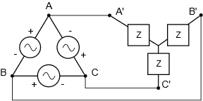
The most straightforward systems are delta-to-delta and Y-to-Y. We shall refer to these as homogeneous systems as the structures of the generator and load are similar. Examples are shown in Figures \(\PageIndex{1}\) and \(\PageIndex{2}\), respectively.

Figure \(\PageIndex{1}\): A delta-connected generator with a delta-connected load (delta-delta).

Figure \(\PageIndex{2}\): A Y-connected generator with a Y-connected load (Y-Y). Optional fourth neutral wire from center to center shown.

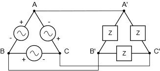
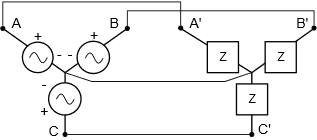
In these configurations, each leg of the load matches up with a corresponding leg of the generator. In the delta-delta configuration of Figure \(\PageIndex{1}\), it should be obvious just by inspection that the voltage across any load leg must equal the voltage of the corresponding generator leg. For example, the load impedance connected between \(A'\) and \(B'\) must see the voltage presented by the generator situated between \(A\) and \(B\) because \(A\) is directly connected to \(A'\) as is \(B\) to \(B'\). Similarly, for the Y-Y configuration of Figure \(\PageIndex{2}\), the current through any load leg must equal the current flowing through the associated generator leg as there are no other paths for current between \(A\) and \(A'\), \(B\) and \(B'\), and \(C\) and \(C'\).

As the load is balanced and the legs of the generator are identical except for their phase, it must be the case that the voltages and currents (and hence the powers) for each leg of the load must be the same, with the exception of the phase. This is true for both the Y-Y configuration as well as the delta-delta configuration. The tricky bit here is the difference between a source (or load) current or voltage, and the line current or voltage.

\[\text{Line voltage is the voltage magnitude between any two conductors connecting the source to the load, excluding ground or common.} \nonumber \]

\[\text{Line current is the current magnitude flowing in any conductor connecting the source to the load, excluding ground or common.} \nonumber \]

Consider the delta-delta system of Figure \(\PageIndex{1}\). We have already established that the voltage developed by generator \(A,B\) must be the same as the voltage across the load \(A',B'\). Thus, the voltage measured from the A, A' conductor to the B,B' conductor must be the same as source and and load voltages. In other words, in the delta-delta configuration, the source, load, and line voltages are all the same.

We also found that the source and load currents must be the same for the delta-delta configuration, however, this does not imply that the current flowing through the wire connecting \(A\) to\(A'\) must be the same as the current flowing through either the generator or the load. After all, two load wires connect to \(A'\), not just one. By definition, the current flowing through that wire is the line current, and therefore in a delta-delta configuration, the line current is not the same as the source or load currents. To avoid confusion, the voltage or current associated with a single leg is referred to as the phase voltage or current versus the line voltage or current.

Turning to the Y-Y configuration of Figure \(\PageIndex{2}\), we see an opposite situation. The source, load, and line currents will all be the same. On the other hand, the line voltage comprises two generators, not one (e.g., from \(A\) to \(B\) or from \(B\) to \(C\)). Thus, for a Y-Y configuration the source and load voltages are the same, but they are not equal to the line voltage (nor is twice, thanks to the phase shift).

Determining Line Voltage and Current

In order to determine the line voltage for a Y-connected generator (and similarly, the line current for a delta connected generator), it is useful to examine a phasor plot of the individual generator voltages. This is shown in Figure \(\PageIndex{3}\). We have three voltages of identical amplitude, the only difference between them being their phase. Each vector is separated from the others by 120 degrees. Further, each individual generator is connected from the common point to one of the external points of \(A\), \(B\) and \(C\). Line voltage is defined as the potential existing between any two if these three points. While it's possible to simply subtract one generator voltage from another to arrive at the difference, there is a nice graphical solution from which we can derive a precise formula for the line voltage given the generator voltage.

Figure \(\PageIndex{3}\): Phasor diagram of Y-connected generator

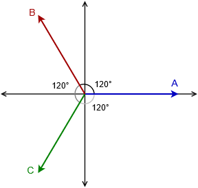
We begin by focusing on quadrants two and three of the phasor plot. This section is redrawn in Figure \(\PageIndex{4}\). In reality, any two vectors can be used for the following proof, but this pair turns out to be particularly convenient in its orientation.

Figure \(\PageIndex{4}\): Solving for the line voltage of a Y-connected generator.

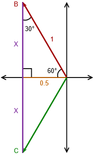
For ease of use we shall normalize the magnitude of the generator voltage to unity. What we see is that the \(B\) and \(C\) vectors are split perfectly by the horizontal axis; that which is above the axis is perfectly mirrored below it. In the upper portion we find a right triangle with a hypotenuse of unity (dark red). The angle it makes with the horizontal must be half of the angle between it and the \(C\) vector. That's half of 120 degrees, or 60 degrees. As the sum of the interior angles of a triangle must be 180 degrees, this means that the third angle must be 30 degrees. The horizontal leg of the triangle (dark yellow or maybe “spicy mustard”) can be determined because we know both the hypotenuse and the opposite angle.

\[\text{opposite } = \text{ hypotenuse }\times \sin \theta \nonumber \]

The sine of 30 degrees is exactly 0.5, therefore, the horizontal leg of the triangle must be 0.5 times the magnitude of unity, or 0.5. We can use the Pythagorean theorem to find the remaining vertical leg (purple).

\[\text{vertical } = \sqrt{\text{hypotenuse}^2−\text{horizontal}^2} \nonumber \]

\[\text{vertical } = \sqrt{1^2−0.5^2} \nonumber \]

\[\text{vertical } = \sqrt{\frac{3}{4}} \nonumber \]

\[\text{vertical } = \frac{1}{2} \sqrt{3} \nonumber \]

The vertical leg is perfectly mirrored below the horizontal axis. Therefore, the span from \(B\) to \(C\) must be twice this value, or \(\sqrt{3}\). As the voltage developed across each leg of the generator is referred to as the generator's phase voltage, we can state:

\[\text{The line voltage for a Y-connected generator is } \sqrt{3} \text{ times its phase voltage.} \label{9.1} \]

For example, if the phase voltage of a Y-connected generator is 120 volts, the line voltage would be \(\sqrt{3}\) times larger, or approximately 208 volts.

For a delta-connected generator, the same holds true for the phase and line currents, with the proof left as an exercise. That is,

\[\text{The line current for a delta-connected generator is } \sqrt{3} \text{ times its phase current.} \label{9.2} \]

These same relationships hold for the loads as well as the sources, e.g., the current in a leg of a Y-connected load will be the same as the line current and its phase voltage will be \(\sqrt{3}\) times smaller than the line voltage.

\[\text{ In summation: For delta configurations (generator or load), the phase voltage is equal to the line voltage while the line current is larger than the phase current by } \sqrt{3} \text{. For Y configurations, the phase current is equal to the line current while the line voltage is } \sqrt{3} \text{ larger than the phase voltage.} \nonumber \]

For homogenous systems, as the generator and load share the same configuration, the phase voltages and currents of the load must be identical to those of the generator. A useful memory aid is that the power dissipated in the system must equal the power generated.

Example \(\PageIndex{1}\)

A three-phase delta-connected generator feeds a three-phase delta-connected load like the system shown in Figure \(\PageIndex{1}\). Assume the generator phase voltage is 120 VAC RMS. The load consists of three identical legs of 50 \( \Omega \) each. Determine the line voltage, load phase voltage, generator phase current, line current, load phase current and the total power delivered to the load.

As this is a homogenous (delta-delta) system, the load phase voltage and current are the same as those of the generator. Therefore, the load phase voltage must also be 120 volts. Second, in a delta configuration, the line voltage equals the phase voltage, again 120 volts. The load phase current is found via Ohm's law and will be an RMS value because the voltage is RMS:

\[i_{phase} = \frac{v_{phase}}{Z_{load}} \nonumber \]

\[i_{phase} = \frac{120 V}{50 \Omega} \nonumber \]

\[i_{phase} = 2.4 A \nonumber \]

The generator's phase current must be the same because the generator and load have the same configuration. For delta configurations, the line current is \(\sqrt{3}\) times larger than the phase current, thus,

\[i_{line} = \sqrt{3}\times i_{phase} \nonumber \]

\[i_{line} = \sqrt{3}\times 2.4A \nonumber \]

\[i_{line} \approx 4.157A \nonumber \]

Finally, total power can be found with a straight application of power law as the load is purely resistive and we have RMS values. Remember, this is three times the power dissipated in one leg.

\[P_{total} = 3\times {i_{phase}}^2 \times R \nonumber \]

\[P_{total} = 3\times (2.4 A)^2\times 50 \Omega \nonumber \]

\[P_{total} = 864 W \nonumber \]

This is equivalent to about 1.2 HP. We could have also computed the load phase power by using the squared phase voltage divided by the load resistance, or by multiplying the phase voltage by the phase current. As this is a purely resistive load, there is no phase angle, and thus no power factor with which to concern ourselves.

Example \(\PageIndex{2}\)

A three-phase Y-connected generator feeds a three-phase Y-connected load similar to the system shown in Figure \(\PageIndex{2}\). Assume the generator phase voltage is 220 VAC RMS. The load consists of three identical legs of 100 \( \Omega \) each. Determine the line voltage, load phase voltage, generator phase current, line current, load phase current and the total power delivered to the load.

This is a homogenous (Y-Y) system, therefore the load phase voltage and current are the same as those of the generator. Consequently, the load phase voltage must be 220 volts. In a Y configuration, the line voltage equals the phase voltage times \(\sqrt{3}\).

\[v_{line} = \sqrt{3}\times v_{phase} \nonumber \]

\[v_{line} = \sqrt{3}\times 220V \nonumber \]

\[v_{line} \approx 381 V \nonumber \]

The load phase current is found via Ohm's law and will be an RMS value because the voltage is RMS. This is the same as the generator phase current and also the line current.

\[i_{phase} = \frac{v_{phase}}{Z_{load}} \nonumber \]

\[i_{phase} = \frac{220 V}{100 \Omega} \nonumber \]

\[i_{phase} = 2.2A \nonumber \]

Total power can be found using basic power law as the load is purely resistive and we have RMS values. In this case we'll use current times voltage for a change of pace.

\[P_{total} = 3\times i_{phase} \times v_{phase} \nonumber \]

\[P_{total} = 3\times 2.2 A\times 220 V \nonumber \]

\[P_{total} = 1452 W \nonumber \]

This is just shy of 2 HP. Once again, this is a purely resistive load and there is no phase angle. Thus, the power factor is unity with the real and apparent powers being the same.

Example \(\PageIndex{3}\)

For the the system shown in Figure \(\PageIndex{5}\), determine the total apparent and real power delivered to the load. Also find the line voltage. The phase voltage of the source is 240 volts RMS at 60 Hz.

Figure \(\PageIndex{5}\): Circuit for Example \(\PageIndex{3}\).

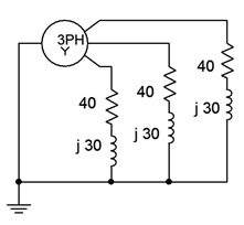
Given the fact that the three load legs are all together at one common point (ground), this must be a Y-Y system. Consequently, we know that the line voltage must be \(\sqrt{3}\) times the phase voltage of the generator.

\[v_{line} = \sqrt{3}\times v_{phase} \nonumber \]

\[v_{line} = \sqrt{3}\times 240 V \nonumber \]

\[v_{line} \approx 416 V RMS \nonumber \]

This is a homogenous system (Y-Y) so we also know that the load voltage is equal to the generator voltage, or 240 volts RMS. From that we can find the load current (the line current must be the same value because this is a Y-connected load).

\[i_{phase} = \frac{v_{phase}}{Z_{load}} \nonumber \]

\[i_{phase} = \frac{240 V}{40+j 30 \Omega} \nonumber \]

\[i_{phase} = 4.8\angle −36.87^{\circ} A \nonumber \]

The phase angle is appropriate for the 0\(^{\circ}\) reference generator. The other two angles will be off of this by \(\pm\)120\(^{\circ}\). The apparent power is simply the product of the load current and voltage magnitudes.

\[S = 3\times i_{load} \times v_{load} \nonumber \]

\[S = 3\times 4.8A\times 240V \nonumber \]

\[S = 3456 VA \nonumber \]

The real power can be found a few different ways:

\[P = S\times \cos \theta \nonumber \]

\[P = 3456 VA \times \cos (−36.87^{\circ}) \nonumber \]

\[P = 2765 W \nonumber \]

\[P = 3\times {i_{load}}^2\times R_{load} \nonumber \]

\[P = 3\times 4.8A 2\times 40 \Omega \nonumber \]

\[P = 2765W \nonumber \]

Computer Simulation

The circuit of Example \(\PageIndex{3}\) is worthy of a simulation. The first thing to do is to determine an appropriate value of inductance to achieve a reactance of \(j40 \Omega \). Given the 60 Hz source frequency, this turns out to be approximately 80 mH. The circuit is constructed as shown in Figure \(\PageIndex{6}\). The 240 volt RMS source phase voltage is equivalent to approximately 340 volts peak. The positions of the inductor and resistor in each leg have been swapped for a reason that will be apparent shortly.

Figure \(\PageIndex{6}\): The equivalent system of Figure \(\PageIndex{5}\) in a simulator.

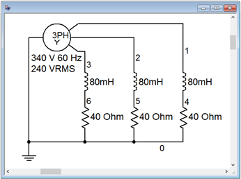
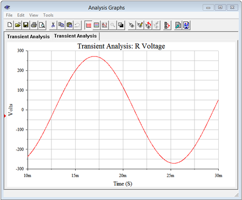
The immediate item of interest is to verify the time shifts and amplitudes of the phase voltages. These correspond to nodes 1, 2 and 3. In this configuration, the load phase voltage equals the generator phase voltage, thus they should be 340 volts peak and separated by 120 degrees or 1/3rd of a cycle.

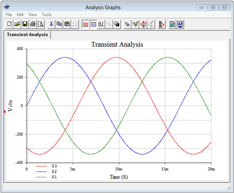
A transient analysis is performed, plotting the node voltages of interest. The result is shown in Figure \(\PageIndex{7}\). The voltages are precisely as expected and the plot compares perfectly to the theoretical plot of Figure 9.2.4.

Figure \(\PageIndex{7}\): The three load voltages simulated from Figure \(\PageIndex{6}\).

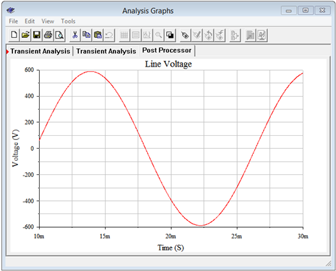
Now we check the line voltage. This was calculated to be 416 volts RMS, or approximately 588 volts peak. The post processor is used to display the result of node voltage 1 minus node voltage 2. This is shown in Figure \(\PageIndex{8}\). Again, the results are as expected with a peak just under 600 volts.

Finally, we will investigate the true load power. Perhaps the easiest way to do this is to determine the voltage across the resistive portion of the load. From prior work we know that true power is only associated with resistance, not reactance. Thus, all we need to do is measure the peak voltage across the resistor. From there, we find its RMS equivalent, square it, and divide by the resistor value. This gives us the true load power in one leg. For the total power we simply triple the result. Obtaining the voltage across the resistor is easy if the resistor is attached to ground. In that case, it's just the voltage at the node to which the resistor is connected. This is why the inductor and resistor positions were swapped in the simulation. As they are in series, it makes no difference to the overall load impedance, however, the new arrangement allows us to obtain the resistor voltage directly instead of having to rely on a differential voltage obtained through the post processor.

Another transient analysis is performed, this time plotting the voltage across one of the load resistors; namely node 4. The result is shown in Figure \(\PageIndex{9}\). The peak of this waveform is measured to be 271.5 volts, or about 192 volts RMS. Squaring this and dividing by 40 \( \Omega \) yields a little over 921 watts per leg, for a total of about 2765 watts, as expected.

Figure \(\PageIndex{8}\): One of the line voltages simulated from Figure \(\PageIndex{6}\).

Figure \(\PageIndex{9}\): Simulated voltage across one of the load resistors in Figure \(\PageIndex{6}\).

Heterogeneous Systems

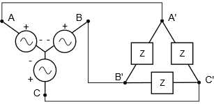
Systems configured as delta-to-Y and Y-to-delta appear to be a bit more complex than homogeneous systems. We shall refer to these as heterogeneous systems as the structures of the generator and load are of opposite kind. Examples are shown in Figures \(\PageIndex{10}\) and \(\PageIndex{11}\), respectively.

Figure \(\PageIndex{10}\): A delta-connected generator with a Y-connected load (delta-Y).

Figure \(\PageIndex{11}\): A Y-connected generator with a delta-connected load (Ydelta).

These systems are not nearly so difficult as some people think; all you have to do is remember statements \ref{9.1} and \ref{9.2}. Indeed, the summation is worth repeating here:

\text{For delta configurations (generator or load), the phase voltage is equal to the line voltage while the line current is larger than the phase current by } \sqrt{3} \text{. For Y configurations, the phase current is equal to the line current while the line voltage is } \sqrt{3} \text{ larger than the phase voltage.} \nonumber \]

You can think of analyzing these systems as a two-step process. First, determine the line voltage and current from either the generator or load; and second, transition from the line to the other side (load or generator). If confusion sets in, remember that power generated must equal power dissipated or delivered.

In Figure \(\PageIndex{10}\), the line voltage equals the generator phase voltage. The load is Yconnected, so each leg sees the line voltage divided by \(\sqrt{3}\). Based on this, each leg of the load current can be computed. Note that the line current equals the load current. The generator phase current will be the line current divided by \(\sqrt{3}\).

In Figure \(\PageIndex{11}\), the line voltage equals \(\sqrt{3}\) times the generator phase voltage. The load is delta-connected, so each leg sees the line voltage. Knowing this, each leg of the load current can be computed. Also, the line current equals the generator phase current, and the load phase current will equal the line current divided by \(\sqrt{3}\).

Example \(\PageIndex{4}\)

A delta-Y system like the one shown in Figure \(\PageIndex{10}\) has a generator phase voltage of 230 volts RMS at 50 Hz. If the load is \(200\angle 0^{\circ}\) \( \Omega \), determine the generator phase current, the line voltage, the load phase voltage, the load phase current and the total power delivered to the load.

The generator is delta connected so the line voltage equals the generator phase voltage, or 230 volts. The load, being Y-connected, will see a phase voltage that is reduced by a factor of \(\sqrt{3}\).

\[v_{load} = \frac{v_{line}}{\sqrt{3}} \nonumber \]

\[v_{load} = \frac{230 V}{\sqrt{3}} \nonumber \]

\[v_{load} \approx 132.8V RMS \nonumber \]

We can use Ohm's law to determine the load phase current.

\[i_{load} = \frac{v_{phase}}{Z_{load}} \nonumber \]

\[i_{load} = \frac{132.8 V}{200\angle 0^{\circ} \Omega} \nonumber \]

\[i_{load} \approx 0.664 A RMS \nonumber \]

Being Y-connected, the line current must be the same as the load phase current, or 0.664 amps. For delta connections, the line current is \(\sqrt{3}\) times larger than the phase current, therefore the generator phase current must be \(\sqrt{3}\) times smaller.

\[i_{gen} = \frac{i_{line}}{\sqrt{3}} \nonumber \]

\[i_{gen} = \frac{0.664A}{\sqrt{3}} \nonumber \]

\[i_{gen} \approx 0.383A RMS \nonumber \]

The load is purely resistive and we have RMS values so the total power can be found via power law (apparent power equals true power in this case).

\[P_{total} = 3\times {i_{load}}^2 \times R \nonumber \]

\[P_{total} = 3\times (0.664A)^2 \times 200 \Omega \nonumber \]

\[P_{total} = 264 W \nonumber \]

As a crosscheck, the power generated is:

\[P_{total} = 3\times i_{gen} \times v_{gen} \nonumber \]

\[P_{total} = 3\times 0.383A\times 230 V \nonumber \]

\[P_{total} = 264 W \nonumber \]

Power generated equals power dissipated.

Example \(\PageIndex{5}\)

A Y-delta system like the one shown in Figure \(\PageIndex{11}\) has a generator phase voltage of 100 volts RMS at 60 Hz. If the load has a magnitude of 50 \( \Omega \) with a lagging power factor of 0.8, determine the generator phase current, the line voltage, the load phase voltage, the load phase current and the total true power delivered to the load.

The Y-connected generator creates a line voltage equal to the generator phase voltage times \(\sqrt{3}\). This is also the load phase voltage as it is delta-connected.

\[v_{line} = \sqrt{3}\times v_{phase} \nonumber \]

\[v_{line} = \sqrt{3}\times 100 V \nonumber \]

\[v_{line} \approx 173.2V RMS \nonumber \]

The delta-connected load will see a phase voltage that is the same as the line voltage, or 173.2 volts. From this we can determine the load current.

\[i_{load} = \frac{v_{phase}}{Z_{load}} \nonumber \]

\[i_{load} = \frac{173.2V}{50 \Omega} \nonumber \]

\[i_{load} \approx 3.464A RMS \nonumber \]

As the load is delta-connected, the line current is the load current times \(\sqrt{3}\). The generator phase current will be the same as the line current.

\[i_{line} = \sqrt{3}\times i_{phase} \nonumber \]

\[i_{line} = \sqrt{3}\times 3.464A \nonumber \]

\[i_{line} = 6 A RMS \nonumber \]

The true load power can be found several ways. First, we can use the \(i^2 R\) form. To do this we need to find the resistive portion of the load. Recall that the power factor is equal to cosine \(\theta\). Therefore the impedance angle is:

\[\theta = \cos^{−1} PF \nonumber \]

\[\theta = \cos^{−1} 0.8 \nonumber \]

\[\theta \approx 36.9^{\circ} \nonumber \]

The real part is:

\[R = Z \cos \theta \nonumber \]

\[R = 50 \Omega \cos 36.9^{\circ} \nonumber \]

\[R = 40 \Omega \nonumber \]

Alternately, we could've just multiplied \(Z\) by \(PF\) to obtain this. Continuing:

\[P_{total} = 3\times {i_{load}}^2 \times R \nonumber \]

\[P_{total} = 3\times (3.464 A)^2\times 40 \Omega \nonumber \]

\[P_{total} = 1440 W \nonumber \]

We could also find the apparent power and use the power factor.

\[P_{total} = 3\times v_{load} \times i_{load} PF \nonumber \]

\[P_{total} = 3\times 173.2V\times 3.464 A\times 0.8 \nonumber \]

\[P_{total} = 1440 W \nonumber \]

As a crosscheck, compare the power dissipated to the power generated.

\[P_{total} = 3\times v_{gen}\times i_{gen}\times PF \nonumber \]

\[P_{total} = 3\times 100V\times 6A\times 0.8 \nonumber \]

\[P_{total} = 1440 W \nonumber \]