
6.2: Nodal Analysis
- Page ID
- 25273

\( \newcommand{\vecs}[1]{\overset { \scriptstyle \rightharpoonup} {\mathbf{#1}} } \)
\( \newcommand{\vecd}[1]{\overset{-\!-\!\rightharpoonup}{\vphantom{a}\smash {#1}}} \)
\( \newcommand{\id}{\mathrm{id}}\) \( \newcommand{\Span}{\mathrm{span}}\)
( \newcommand{\kernel}{\mathrm{null}\,}\) \( \newcommand{\range}{\mathrm{range}\,}\)
\( \newcommand{\RealPart}{\mathrm{Re}}\) \( \newcommand{\ImaginaryPart}{\mathrm{Im}}\)
\( \newcommand{\Argument}{\mathrm{Arg}}\) \( \newcommand{\norm}[1]{\| #1 \|}\)
\( \newcommand{\inner}[2]{\langle #1, #2 \rangle}\)
\( \newcommand{\Span}{\mathrm{span}}\)
\( \newcommand{\id}{\mathrm{id}}\)
\( \newcommand{\Span}{\mathrm{span}}\)
\( \newcommand{\kernel}{\mathrm{null}\,}\)
\( \newcommand{\range}{\mathrm{range}\,}\)
\( \newcommand{\RealPart}{\mathrm{Re}}\)
\( \newcommand{\ImaginaryPart}{\mathrm{Im}}\)
\( \newcommand{\Argument}{\mathrm{Arg}}\)
\( \newcommand{\norm}[1]{\| #1 \|}\)
\( \newcommand{\inner}[2]{\langle #1, #2 \rangle}\)
\( \newcommand{\Span}{\mathrm{span}}\) \( \newcommand{\AA}{\unicode[.8,0]{x212B}}\)
\( \newcommand{\vectorA}[1]{\vec{#1}} % arrow\)
\( \newcommand{\vectorAt}[1]{\vec{\text{#1}}} % arrow\)
\( \newcommand{\vectorB}[1]{\overset { \scriptstyle \rightharpoonup} {\mathbf{#1}} } \)
\( \newcommand{\vectorC}[1]{\textbf{#1}} \)
\( \newcommand{\vectorD}[1]{\overrightarrow{#1}} \)
\( \newcommand{\vectorDt}[1]{\overrightarrow{\text{#1}}} \)
\( \newcommand{\vectE}[1]{\overset{-\!-\!\rightharpoonup}{\vphantom{a}\smash{\mathbf {#1}}}} \)
\( \newcommand{\vecs}[1]{\overset { \scriptstyle \rightharpoonup} {\mathbf{#1}} } \)
\( \newcommand{\vecd}[1]{\overset{-\!-\!\rightharpoonup}{\vphantom{a}\smash {#1}}} \)
\(\newcommand{\avec}{\mathbf a}\) \(\newcommand{\bvec}{\mathbf b}\) \(\newcommand{\cvec}{\mathbf c}\) \(\newcommand{\dvec}{\mathbf d}\) \(\newcommand{\dtil}{\widetilde{\mathbf d}}\) \(\newcommand{\evec}{\mathbf e}\) \(\newcommand{\fvec}{\mathbf f}\) \(\newcommand{\nvec}{\mathbf n}\) \(\newcommand{\pvec}{\mathbf p}\) \(\newcommand{\qvec}{\mathbf q}\) \(\newcommand{\svec}{\mathbf s}\) \(\newcommand{\tvec}{\mathbf t}\) \(\newcommand{\uvec}{\mathbf u}\) \(\newcommand{\vvec}{\mathbf v}\) \(\newcommand{\wvec}{\mathbf w}\) \(\newcommand{\xvec}{\mathbf x}\) \(\newcommand{\yvec}{\mathbf y}\) \(\newcommand{\zvec}{\mathbf z}\) \(\newcommand{\rvec}{\mathbf r}\) \(\newcommand{\mvec}{\mathbf m}\) \(\newcommand{\zerovec}{\mathbf 0}\) \(\newcommand{\onevec}{\mathbf 1}\) \(\newcommand{\real}{\mathbb R}\) \(\newcommand{\twovec}[2]{\left[\begin{array}{r}#1 \\ #2 \end{array}\right]}\) \(\newcommand{\ctwovec}[2]{\left[\begin{array}{c}#1 \\ #2 \end{array}\right]}\) \(\newcommand{\threevec}[3]{\left[\begin{array}{r}#1 \\ #2 \\ #3 \end{array}\right]}\) \(\newcommand{\cthreevec}[3]{\left[\begin{array}{c}#1 \\ #2 \\ #3 \end{array}\right]}\) \(\newcommand{\fourvec}[4]{\left[\begin{array}{r}#1 \\ #2 \\ #3 \\ #4 \end{array}\right]}\) \(\newcommand{\cfourvec}[4]{\left[\begin{array}{c}#1 \\ #2 \\ #3 \\ #4 \end{array}\right]}\) \(\newcommand{\fivevec}[5]{\left[\begin{array}{r}#1 \\ #2 \\ #3 \\ #4 \\ #5 \\ \end{array}\right]}\) \(\newcommand{\cfivevec}[5]{\left[\begin{array}{c}#1 \\ #2 \\ #3 \\ #4 \\ #5 \\ \end{array}\right]}\) \(\newcommand{\mattwo}[4]{\left[\begin{array}{rr}#1 \amp #2 \\ #3 \amp #4 \\ \end{array}\right]}\) \(\newcommand{\laspan}[1]{\text{Span}\{#1\}}\) \(\newcommand{\bcal}{\cal B}\) \(\newcommand{\ccal}{\cal C}\) \(\newcommand{\scal}{\cal S}\) \(\newcommand{\wcal}{\cal W}\) \(\newcommand{\ecal}{\cal E}\) \(\newcommand{\coords}[2]{\left\{#1\right\}_{#2}}\) \(\newcommand{\gray}[1]{\color{gray}{#1}}\) \(\newcommand{\lgray}[1]{\color{lightgray}{#1}}\) \(\newcommand{\rank}{\operatorname{rank}}\) \(\newcommand{\row}{\text{Row}}\) \(\newcommand{\col}{\text{Col}}\) \(\renewcommand{\row}{\text{Row}}\) \(\newcommand{\nul}{\text{Nul}}\) \(\newcommand{\var}{\text{Var}}\) \(\newcommand{\corr}{\text{corr}}\) \(\newcommand{\len}[1]{\left|#1\right|}\) \(\newcommand{\bbar}{\overline{\bvec}}\) \(\newcommand{\bhat}{\widehat{\bvec}}\) \(\newcommand{\bperp}{\bvec^\perp}\) \(\newcommand{\xhat}{\widehat{\xvec}}\) \(\newcommand{\vhat}{\widehat{\vvec}}\) \(\newcommand{\uhat}{\widehat{\uvec}}\) \(\newcommand{\what}{\widehat{\wvec}}\) \(\newcommand{\Sighat}{\widehat{\Sigma}}\) \(\newcommand{\lt}{<}\) \(\newcommand{\gt}{>}\) \(\newcommand{\amp}{&}\) \(\definecolor{fillinmathshade}{gray}{0.9}\)Nodal analysis can be considered a universal solution technique as there are no practical circuit configurations that it cannot handle. It does not matter if there are multiple sources or if there are complex configurations that cannot be reduced using series-parallel simplification techniques, nodal analysis can handle them all. Further, nodal analysis tends to “give us what we want”, namely, a set of node voltages for the circuit. Once the node voltages are obtained, finding any branch currents or component powers becomes an almost trivial exercise. Nodal analysis relies on the application of Kirchhoff's current law to create a series of node equations that can be solved for node voltages. These equations are based on Ohm's law and will be of the form \(i = v/Z\), or more generally, \(i = (1/Z_X) \cdot v_A + (1/Z_Y) \cdot v_B + (1/Z_Z) \cdot v_C \dots\)
We will examine two variations on the theme; first, a general version that can be used with both voltage and current sources, and a second somewhat quicker version that can be used with circuits only driven by current sources.
General Method
Consider the circuit shown in Figure \(\PageIndex{1}\). We begin by labeling connection nodes. We are interested in identifying current junctions, that is, places where currents can combine or split. These are also known as summing nodes and are circled in blue on the figure. We do not concern ourselves with points where just two components connect without any other connection, such as points \(a\) and \(c\). Once the proper nodes are identified, reference current directions are assigned. The reference current directions are chosen arbitrarily and for convenience. They may be the opposite of reality. This is not a problem. If we assign directions that are reversed, we'll simply wind up with a current version of a double negative, and the computed node voltages will work out just fine.
One node is chosen as the reference. This is the point to which all other node voltages are measured against. Typically, the reference node is ground, although it does not have to be.
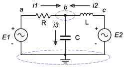
We now write a current summation equation for each summing node, except for the reference node. In this circuit there is only one node where currents combine (other than ground) and that's node \(b\). Points \(a\) and \(c\) are places where components connect, but they are not summing nodes, so we can ignore them for now. Using KCL on node \(b\) we can say:
\[i_1 + i_2 = i_3 \nonumber \]
Now we'll describe these currents in terms of the source and node voltages, and associated components. For example, \(i_3\) is the node \(b\) voltage divided by \(−jX_C\) while \(i_1\) is the voltage across \(R\) divided by \(R\). This voltage is \(v_a − v_b\).
\[ \frac{v_a −v_b}{R} + \frac{v_c −v_b}{jX_L} = \frac{v_b}{-jX_C} \nonumber \]
Noting that \(v_a = E_1\) and \(v_c = E_2\), with a little algebra this can be reduced to:
\[\left( \frac{1}{R} \right) E_1 + \left( \frac{1}{jX_L} \right) E_2 = \left( \frac{1}{R} + \frac{1}{jX_L} + \frac{1}{-jX_C} \right) v_b \nonumber \]
All quantities are known except for \(v_b\) and thus it is easily found with a little more algebra. If there had been more nodes, there would have been more equations and more unknowns, one for each node. As we shall see, this conductance-voltage product format turns out to be a convenient way of writing these equations. Also, note that the first two terms on the left reduce to fixed current values.
For current sources, the process is similar but a bit more direct. Consider the circuit of Figure \(\PageIndex{2}\). We start as before, identifying nodes and labeling currents. We then write the current summation equations at each node (except for ground). We consider currents entering a node as positive and exiting as negative. There are two nodes of interest here, and thus, two equations each with two unknowns will be generated.
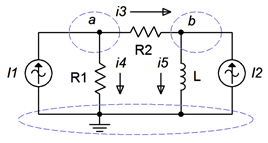
Node \(a\): \(I_1 = i_3 + i_4\)
Node \(b\): \(i_3 + I_2 = i_5\), and rearranging in terms of the fixed source,
Node \(b\): \(I_2 = −i_3 + i_5\)
The currents are then described by their Ohm's law equivalents:
Node \(a\): \(I_1 = \frac{v_a −v_b}{R_2} + \frac{v_a}{R_1}\)
Node \(b\): \(I_2 = − \frac{v_a −v_b}{R_2} + \frac{v_b}{jX_L}\)
Expanding and collecting terms yields:
Node \(a\): \(I_1 = \left( \frac{1}{R_1} + \frac{1}{R_2} \right) v_a − \left( \frac{1}{R_2} \right) v_b \)
Node \(b\): \(I_2 = − \left( \frac{1}{R_2} \right) v_a + \left( \frac{1}{R_2} + \frac{1}{jX_L} \right) v_b \)
As the impedance values and currents are known, simultaneous equation solution techniques may be used to solve for the node voltages. Once again, there are as many equations as node voltages.
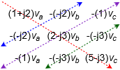
One practical point before continuing: It is very important that the coefficients for the various node voltage terms “line up” when the final system of equations is written out. That is, there should be a column for the \(v_a\) terms, a column for the \(v_b\) terms, and so on. They should not be written out in random order, but rather following the style shown in Figure \(\PageIndex{3}\). This format will make it much it easier to enter the coefficients into a calculator or solve manually. Further, the set of coefficients must show diagonal symmetry. That is, if we draw a major diagonal from upper-left to lower-right (red), whatever coefficients are above-right from the diagonal should be mirrored below-left of the diagonal (blue, purple, green). If the set of values does not show diagonal symmetry, an error has been made. You must go back and recheck the original node summations. Simple as that. Even the simple 2x2 of Figure \(\PageIndex{2}\) shows this symmetry (namely, the coefficient of \(−1/R_2\) for \(v_b\) in the first equation and \(v_a\) in the second).
Example \(\PageIndex{1}\)
Determine the voltage across the inductor in the circuit of Figure \(\PageIndex{4}\). Source one is \(5 \angle 0^{\circ}\) volts RMS and source two \(2 \angle 90^{\circ}\) volts RMS.
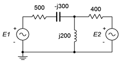
Other than ground, there is only one current summing node in this circuit, and that's the junction at the top of the inductor. We will refer to this junction as node \(a\). Following the outline of Figure \(\PageIndex{1}\), we define three currents; \(i_1\) entering from the left, \(i_2\) entering from the right, and \(i_3\) exiting down through the inductor.
\[i_1 + i_2 = i_3 \nonumber \]
Next, these currents are described in terms of the voltages and components. We'll number the resistors from left to right.
\[\frac{E_1 − v_a}{R_1 − jX_C} + \frac{E_2 − v_a}{R_2} = \frac{v_a}{jX_L} \nonumber \]
This can be rearranged as:
\[\left( \frac{1}{R_1 − jX_C} \right) E_1 + \left( \frac{1}{R_2} \right) E_2 = \left( \frac{1}{R_1 − jX_C} + \frac{1}{R_2} + \frac{1}{jX_L} \right) v_a \nonumber \]
Populate with values:
\[\left( \frac{1}{500 − j 300\Omega} \right) 5 \angle 0^{\circ} V + \left( \frac{1}{400 \Omega} \right) 2 \angle 90^{\circ} V = \left( \frac{1}{500− j 300\Omega} + \frac{1}{400 \Omega} + \frac{1}{j 200\Omega} \right) v_a \nonumber \]
This simplifies to:
\[8.575E-3 \angle 31^{\circ} A +5E-3 \angle 90^{\circ} A = (5.72E-3 \angle −46^{\circ} S) v_a \nonumber \]
Solving for the unknown, we find that \(v_a = 2.087 \angle 98^{\circ}\) volts RMS.
Example \(\PageIndex{2}\)
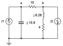
In the circuit of Figure \(\PageIndex{5}\), determine \(v_a\) and \(v_b\). \(E\) is \(20 \angle 0^{\circ}\) volts peak while \(I\) is \(0.1 \angle 0^{\circ}\) amps peak. The system frequency is 2 kHz.
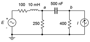
There are two nodes of interest here, other than ground. This means we will generate two equations with two unknowns (\(v_a\) and \(v_b\)). Using the standard reactance formulas, the inductive and capacitive reactances are found to be \(j125.7 \Omega \) and \(−j159.2 \Omega \), respectively. If we assume the reference direction for current is from node \(a\) to node \(b\), and that the current flow through the two center resistors is downward, the equations are:
Node \(a\): \(\frac{20 \angle 0^{\circ} V −v_a}{100+j 125.7\Omega} = \frac{v_a}{250\Omega} + \frac{v_a −v_b}{− j 159.2 \Omega}\)
Node \(b\): \(\frac{v_a −v_b}{− j159.2 \Omega} +0.1 \angle 0^{\circ} A = \frac{v_b}{400\Omega}\)
Expanding and collecting terms yields:
Node \(a\): \(0.1245 \angle −51.5^{\circ} A = \left( \frac{1}{250\Omega} + \frac{1}{100+j 125.7\Omega} + \frac{1}{− j 159.2 \Omega} \right) v_a − \left( \frac{1}{− j 159.2\Omega} \right) v_b \)
Node \(b\): \(0.1 \angle 0^{\circ} A = − \left( \frac{1}{− j 159.2\Omega} \right) v_a + \left( \frac{1}{400\Omega} + \frac{1}{− j 159.2\Omega} \right) v_b\)
These are simplified, ready for manipulation (note diagonal symmetry).
\[0.1245 \angle −51.5^{\circ} A = ( 8E-3 \angle 10.1^{\circ} S) v_a − (6.281E-3 \angle 90^{\circ} S) v_b \nonumber \]
\[0.1 \angle 0^{\circ} A =− (6.281E-3 \angle 90^{\circ} S) v_a +(6.76E-3 \angle 68.3^{\circ} S)v_b \nonumber \]
After solving the system of equations, we see that \(v_a = 16.24 \angle 0.09^{\circ}\) volts and \(v_b = 20.99 \angle −22.3^{\circ}\) volts.
Computer Simulation
To verify the results of the preceding example, the circuit of Figure \(\PageIndex{5}\) is captured in a simulator as shown in Figure \(\PageIndex{6}\).
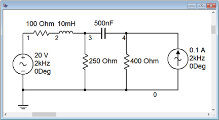
A transient analysis is performed on the circuit. Node voltages 1, 3 and 4 are plotted, corresponding to the voltage source and nodes \(a\) and \(b\), respectively, in Figure \(\PageIndex{7}\).
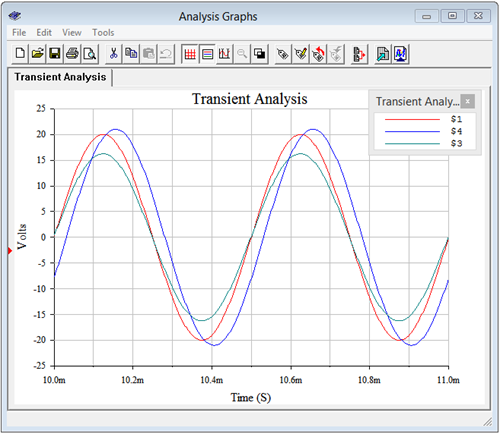
The amplitudes are just as computed. Node voltage \(a\) appears to be nearly in phase with the voltage source, as expected. Node voltage \(b\) lags the source by between one-quarter to one-third of a division, or some 30 microseconds. For a 2 kHz source, this translates to around −22 degrees, verifying the calculated result.
Example \(\PageIndex{3}\)
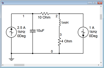
For the circuit of Figure \(\PageIndex{8}\), find \(v_a\) and \(v_b\). The system frequency is 1 kHz. \(I_1 = 2.5 \angle 0^{\circ}\) A and \(I_2 = 1 \angle 0^{\circ}\) A.
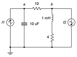
We will generate two equations with two unknowns, \(v_a\) and \(v_b\). The reactance formulas yield \(j6.28 \Omega \) and \(−j15.9 \Omega \) for the inductor and capacitor. If we assume the reference direction for current is from node \(a\) to node \(b\), and that the current flow through the capacitor and inductor is from nodes \(a\) and \(b\) downward, the equations are:
Node \(a\): \(2.5 \angle 0^{\circ} A = \frac{v_a}{− j 15.9\Omega} + \frac{v_a −v_b}{10 \Omega} \)
Node \(b\): \(\frac{v_a −v_b}{10\Omega} = 1 \angle 0^{\circ} A + \frac{v_b}{4+j 6.28\Omega} \)
Expanding and collecting terms yields (note diagonal symmetry):
\[2.5 \angle 0^{\circ} A = \left( \frac{1}{10\Omega} +\frac{1}{− j 15.9\Omega} \right) v_a − \left( \frac{1}{10\Omega} \right) v_b \nonumber \]
\[−1 \angle 0^{\circ} A = − \left( \frac{1}{10\Omega} \right) v_a + \left( \frac{1}{10\Omega} + \frac{1}{4 +j 6.28\Omega} \right) v_b \nonumber \]
\[2.5 \angle 0^{\circ} A = (0.118 \angle 32.2^{\circ} S) v_a − (0.1 \angle 0^{\circ} S) v_b \nonumber \]
\[−1 \angle 0^{\circ} A = − (0.1 \angle 0^{\circ} S) v_a +(0.206 \angle −33.3^{\circ} S) v_b \nonumber \]
The results are: \(v_a = 30.39 \angle -38.7^{\circ}\) volts and \(v_b = 11.37 \angle −20.8^{\circ}\) volts.
Computer Simulation
To verify the results of the preceding example, the circuit of Figure \(\PageIndex{8}\) is captured in a simulator as shown in Figure \(\PageIndex{9}\).
A transient analysis is performed on the circuit. Node voltages 1 and 2 (i.e., nodes \(a\) and \(b\), respectively) are plotted in Figure \(\PageIndex{10}\).
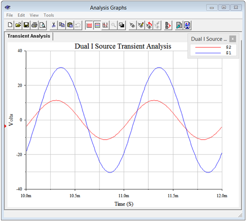
The simulation results agree nicely with the computed values in terms of both amplitude and phase.
Inspection Method
The system of equations can be obtained directly through inspection if the circuit contains current sources and no voltage sources. Let's take another look at the equations developed in the preceding example. For convenience, the circuit is reproduced in Figure \(\PageIndex{11}\) with reactance values. \(I_1 = 2.5 \angle 0^{\circ}\) A and \(I_2 = 1 \angle 0^{\circ}\) A.
\[2.5 \angle 0^{\circ} A = \left( \frac{1}{10\Omega} + \frac{1}{− j 15.9\Omega} \right) v_a − \left( \frac{1}{10\Omega} \right) v_b \nonumber \]
\[−1 \angle 0^{\circ} A = − \left( \frac{1}{10\Omega} \right) v_a + \left( \frac{1}{10\Omega} + \frac{1}{4 +j 6.28\Omega} \right) v_b \nonumber \]
The top equation was built around a current summation at node \(a\) while the bottom was built around a summation at node \(b\). The first thing that might be apparent is that on the left of the equals signs are the current sources connected to these nodes. Positive means the current is entering while negative denotes an exiting current. The second thing is that, for the node of interest (node \(a\) for the top equation, node \(b\) for the bottom), the coefficients represent the items connected to that particular node. For example, in the top equation, the components connected to node \(a\) are the 10 \(\Omega \) resistor and the \(− j15.9 \Omega \) reactance. Likewise, in the bottom equation, the components connected to node \(b\) are the 10 \(\Omega \) resistor and the \(4 + j6.28 \Omega \) impedance. The third thing is that the remaining coefficients consist of the components that are in common between the node of interest and the other node (i.e., 10 \(\Omega \) connects \(a\) to \(b\) for the first equation, and also connects \(b\) to \(a\) for the second equation). These other connections always show up as negative. The reason for this should be apparent if you examine the structure of the original equations from Example \(\PageIndex{3}\).
If there is no bridging element between a node and the node of interest, then that coefficient will be zero. If voltage sources exist in the circuit, source conversions can be used to obtain an equivalent circuit that uses only current sources.
The huge advantage of the inspection method is that it cuts out a time consuming and error prone section of the process, namely converting the original KCL summations into a set of simplified equations with coefficients for each unknown. The inspection method generates the equations directly. To further speed the process, it can be useful to turn each impedance value into a corresponding admittance value before creating the equations. In this way, the reciprocals are computed once for each item rather than multiple times in multiple equations. Finally, remember that the resulting set of equations must exhibit diagonal symmetry, as shown back in Figure \(\PageIndex{3}\).
The inspection method is summarized as follows:
1. Verify that the circuit uses only current sources and no voltage sources. If voltage sources exist, they must be converted to current sources before proceeding.
2. Find all of the current summing nodes and number (or letter) them. Also decide on the reference node (usually ground).
3. To generate an equation, locate the first node. This is the node of interest and the next few steps will be associated with it.
4. Sum the current sources feeding the node of interest. Entering is deemed positive while exiting is deemed negative. The sum is placed on one side of the equals sign.
5. Next, find all of the impedances connected to the node of interest and write them as a sum of admittances on the other side of the equals sign, the group being multiplied by this node's voltage (e.g., \(v_1\)). That makes one term.
6. Now for the other terms. Find all of the admittances that are connected between the node of interest and the next node (e.g., node 2). Sum these together and multiply the group by this other node's voltage (e.g., \(v_2\)). Subtract that product from the equation built so far. Repeat this process until all of the other nodes have been examined (except ground). If there are no common impedances between the node of interest and the other node, use zero for the coefficient of that node's voltage. Once all other nodes are considered, this equation is finished.
7. Go to the next node and treat this as the new node of interest.
8. Repeat steps 4 through 7 until all nodes have been treated as the node of interest. Each iteration creates a new equation. There will be as many equations as there are nodes, less the reference node. Check for diagonal symmetry and solve.
The inspection method is best observed in action, and is used in the following example.
Example \(\PageIndex{4}\)
Write the system of equations for the circuit of Figure \(\PageIndex{12}\). \(I_1 = 10 \angle 0^{\circ}\) A and \(I_2 = 4 \angle 90^{\circ}\) A.
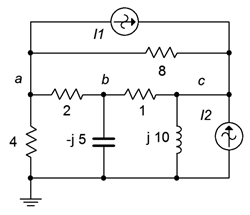
We begin at node \(a\), the first node of interest. Find all of the current sources connected to this node. All we have is \(I_1\). It is exiting, and thus negative.
\[−10 \angle 0^{\circ} A = \dots \nonumber \]
Now find all of the items connected to this node and create a sum of admittances.
\[−10 \angle 0^{\circ} A = \left( \frac{1}{4\Omega} + \frac{1}{2\Omega} + \frac{1}{8\Omega} \right) v_a \dots \nonumber \]
Include the terms that are common between node \(a\) and node \(b\). This is negative.
\[−10 \angle 0^{\circ} A = \left( \frac{1}{4\Omega} + \frac{1}{2\Omega} + \frac{1}{8\Omega} \right) v_a − \left( \frac{1}{2\Omega} \right) v_b \dots \nonumber \]
And finally, include the terms common between node \(a\) and node \(c\). This is also negative.
\[−10 \angle 0^{\circ} A = \left( \frac{1}{4\Omega} + \frac{1}{2\Omega} + \frac{1}{8\Omega} \right) v_a − \left( \frac{1}{2\Omega} \right) v_b − \left( \frac{1}{8\Omega} \right) v_c \nonumber \]
The first equation is done. We now make node \(b\) the node of interest and repeat the process.
Find all of the current sources connected to this node. There are none.
\[0 = \dots \nonumber \]
Find all of the items connected to this node and create a sum of admittances.
\[0 = \dots + \left( \frac{1}{1\Omega} + \frac{1}{2\Omega} + \frac{1}{− j 5\Omega} \right) v_b \dots \nonumber \]
Include the terms that are common between node \(a\) and node \(b\). This is negative and goes into the lead (a before b) to keep everything nicely lined up.
\[0 =− \left( \frac{1}{2\Omega} \right) v_a + \left( \frac{1}{1\Omega} + \frac{1}{2\Omega} + \frac{1}{− j 5\Omega} \right) v_b \dots \nonumber \]
Now include the terms common between node \(b\) and node \(c\). This is also negative and is inserted at the tail (c after b).
\[0 =− \left( \frac{1}{2\Omega} \right) v_a + \left( \frac{1}{1\Omega} + \frac{1}{2\Omega } + \frac{1}{− j 5\Omega} \right) v_b − \left( \frac{1}{1\Omega} \right) v_c \nonumber \]
The second equation is finished. We now make node \(c\) the node of interest and repeat the process for the final time. Find all of the current sources connected to node \(c\). We have both \(I_1\) and \(I_2\) entering.
\[10 \angle 0^{\circ} A+4 \angle 90^{\circ} A = \dots \nonumber \]
This current is equivalent to \(10.77 \angle 21.8^{\circ}\). Now find all of the items connected to this node and create a sum of admittances.
\[10.77 \angle 21.8^{\circ} A = \dots \left( \frac{1}{1\Omega} + \frac{1}{8\Omega} + \frac{1}{j 10\Omega} \right) v_c \nonumber \]
Include the terms that are common between node \(c\) and node \(a\). This is negative and goes into the lead (a before c).
\[10.77 \angle 21.8^{\circ} A =− \left( \frac{1}{8\Omega} \right) v_a \dots + \left( \frac{1}{1\Omega} + \frac{1}{8\Omega} + \frac{1}{j 10 \Omega} \right) v_c \nonumber \]
Now include the terms common between node \(b\) and node \(c\). This is also negative and is inserted in the middle (b before c).
\[10.77 \angle 21.8^{\circ} A =−\left( \frac{1}{8\Omega} \right) v_a − \left( \frac{1}{1\Omega} \right) v_b + \left( \frac{1}{1\Omega} + \frac{1}{8\Omega} + \frac{1}{j 10 \Omega} \right) v_c \nonumber \]
The third and final equation is finished. The completed set of equations is:
\[−10 \angle 0^{\circ} A = \left( \frac{1}{4\Omega} + \frac{1}{2\Omega} + \frac{1}{8\Omega} \right) v_a − \left( \frac{1}{2\Omega} \right) v_b − \left( \frac{1}{8\Omega} \right) v_c \nonumber \]
\[0 =− \left( \frac{1}{2\Omega} \right) v_a + \left( \frac{1}{1\Omega} + \frac{1}{2\Omega} + \frac{1}{− j 5\Omega} \right) v_b −\left( \frac{1}{1\Omega} \right) v_c \nonumber \]
\[10.77 \angle 21.8^{\circ} A =− \left( \frac{1}{8\Omega} \right) v_a −\left( \frac{1}{1\Omega} \right) v_b +\left( \frac{1}{1\Omega} + \frac{1}{8\Omega} + \frac{1}{j 10\Omega} \right) v_c \nonumber \]
Note that the set exhibits diagonal symmetry and that all coefficient groups are negative except for those along the major diagonal. Consequently, the coefficient groups may now be simplified to obtain single coefficients for the unknowns, and the equations are ready for solution. The results are: \(v_a = 10.9 \angle 72.8^{\circ}\) volts, \(v_b = 23.6 \angle 34.7^{\circ}\) volts and \(v_c = 31.2 \angle 37.3^{\circ}\) volts. These values can be crosschecked by using them to find the currents through each component, and then verifying KCL for each node.
Although this example may appear to be somewhat long winded, with a little practice the process will become second nature. At that point, the set of equations can be created quickly and with little possibility of error, even for large circuits with many nodes.
Using Source Conversions
As mentioned previously, given circuits with voltage sources, it may be easier to convert them to current sources and then apply the inspection technique rather than using the general approach outlined initially. There is one trap to watch out for when using source conversions: the voltage across or current through a converted component will most likely not be the same as the voltage or current in the original circuit. This is because the location of the converted component will have changed. For example, the circuit of Figure \(\PageIndex{5}\) (Example \(\PageIndex{2}\)) could be solved using the inspection method of nodal analysis by converting the voltage source and its associated impedance of the 100 \Omega resistor in series with the 10 mH inductor into a current source. Although the associated impedance still connects to the converted source, the other end no longer connects to node \(a\). Rather, it would connect to ground. Therefore, the voltage drop across this impedance in the converted circuit is not likely to equal the voltage drop seen across it in the original circuit (the only way they would be equal is if the voltage source \(E\) turned out to be 0).
Supernode
From time to time you may see a circuit utilizing an ideal voltage source like the one shown in Figure \(\PageIndex{13}\). That is, this voltage source does not have a series impedance associated with it. Without that impedance, it becomes impossible to create an expression for the current passing through the source using the general method, and impossible to convert the voltage source into a current source in order to use the inspection method. There are a few of ways out of this quandary. The first way is to recognize that all realistic sources have some internal impedance, so we simply add a very small resistor in series with the source so that a source conversion is possible. Of course, not just any resistor will do. In order to maintain accuracy, the newly added resistance has to be much smaller than any surrounding resistances or reactances. A reduction by two orders of magnitude generally yields a variation smaller than that produced by component tolerances in all but high precision circuits and will usually do the trick. Still smaller values will further increase accuracy. Another way out is to use a supernode.
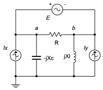
A supernode is, in effect, the combination of two nodes. It relies on a simple observation. If we examine the circuit of Figure \(\PageIndex{13}\), the path of the voltage source produces identical currents flowing into and out of nodes \(a\) and \(b\). As a consequence, if we treat the two nodes as one big node, then when we write a KCL summation, these two terms will cancel. To see just how this works, refer to Figure \(\PageIndex{14}\).
In this version we have replaced the voltage source with its ideal internal impedance; a short. We have also labeled the two nodes of interest, \(a\) and \(b\), and labeled the currents, drawn with convenient reference directions. The specific choice of direction will not matter, just use whatever scheme seems appropriate.
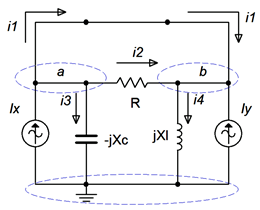
Due to the shorted voltage source, nodes \(a\) and \(b\) are now the same node. Take a look at the currents entering and exiting this combined “super” node. On the left side (formerly node \(a\)) we see a constant current \(I_x\) entering while \(i_1\), \(i_2\) and \(i_3\) are exiting. On the right side (formerly node \(b\)) we see the \(I_y\) entering along with \(i_1\) and \(i_2\), and exiting we see \(i_4\). At this point we'll create an expression where all of currents entering the super node are on the left side of the equals sign and all of the exiting currents are on the right:
\[\sum i_{in} = \sum i_{out} \nonumber \]
\[I_x+ I_y+i_1+i_2 = i_1+i_2+i_3+i_4 \nonumber \]
This can be simplified to:
\[I_x+ I_y = i_3 +i_4 \nonumber \]
Writing this in terms of Ohm's law we have:
\[I_x+I_y = \frac{1}{− j X_C} v_a + \frac{1}{j X_L} v_b \nonumber \]
We also know that \(v_a − v_b = E\) from the original circuit. We know this because the reference polarity of the source is + toward the \(a\) node and − toward the \(b\) node. Therefore it must be \(v_a − v_b\) and not \(v_b − v_a\). Assuming all sources and components are known, that makes two equations with two unknowns, solvable using simultaneous equation techniques. This is illustrated in the following example.
Example \(\PageIndex{5}\)
Find \(v_a\) and \(v_b\) for the circuit of Figure \(\PageIndex{15}\). \(E = 16 \angle 0^{\circ}\) volts, \(I_x = 0.1 \angle 0^{\circ}\) amps and \(I_y = 0.25 \angle 90^{\circ}\) amps.
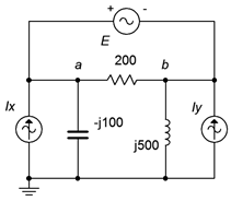
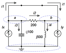
The circuit is redrawn in Figure \(\PageIndex{16}\) with nodes and currents labeled. We short the 16 volt source and write a current summation at the \(a:b\) supernode:
\[\sum i_{in} = \sum i_{out} \nonumber \]
\[0.1 \angle 0^{\circ} A+0.25 \angle 90^{\circ} A +i_1 + i_2 = i_1+i_2+i_3+i_4 \nonumber \]
This can be simplified to:
\[0.2693 \angle 68.2^{\circ} A = i_3 +i_4 \nonumber \]
Writing this in terms of Ohm's law we have:
\[0.2693 \angle 68.2^{\circ} A = \frac{1}{− j 100 \Omega} v_a + \frac{1}{j 500\Omega} v_b \nonumber \]
\[0.2693 \angle 68.2^{\circ} A = j 10 mS v_a − j 2 mS v_b \nonumber \]
We also know that \(v_a − v_b = 16 \angle 0^{\circ}\) volts. Therefore \(v_b = v_a − 16 \angle 0^{\circ}\) volts. Substituting this into the prior equation yields:
\[0.2693 \angle 68.2^{\circ} A = j 10 mSv_a − j2 mS(v_a −16 \angle 0^{\circ} V) \nonumber \]
\[0.2693 \angle 68.2^{\circ} A = j 10 mS v_a − j2 mSv_a +32E-3 \angle 90^{\circ} A \nonumber \]
\[0.2394 \angle 67.9^{\circ} A = j 8 mSv_a \nonumber \]
\[v_a = 29.92 \angle −22.1^{\circ} V \nonumber \]
We know that \(v_b\) is \(16 \angle 0^{\circ}\) volts below \(v_a\), and thus after subtracting, we find \(v_b = 16.24 \angle −43.8^{\circ}\) volts.
To verify, we will perform a KCL summation at each node. For node \(a\), assuming \(i_1\) exits as drawn:
\[i_1 = 0.1 \angle 0^{\circ} A − \frac{v_a}{− j 100\Omega} − \frac{v_a−v_b}{200 \Omega} \nonumber \]
\[i_1 = 0.1 \angle 0^{\circ} A− \frac{29.92 \angle −22.1^{\circ} V}{− j 100 \Omega} − \frac{29.92 \angle −22.1^{\circ} V−16.24 \angle −43.8^{\circ} V}{200 \Omega} \nonumber \]
\[i_1 = 0.292 \angle −108^{\circ} A \nonumber \]
Doing likewise for node \(b\), and assuming \(i_1\) enters as drawn:
\[i_1 =−0.25 \angle 90^{\circ} A + \frac{v_b}{j 500 \Omega} − \frac{v_a−v_b}{20 \Omega} \nonumber \]
\[i_1 =−0.25 \angle 90^{\circ} A + \frac{16.24 \angle −43.8^{\circ} V}{j 500 \Omega} − \frac{29.92 \angle −22.1^{\circ} V −16.24 \angle −43.8^{\circ} V}{200\Omega} \nonumber \]
\[ i_1 = 0.292 \angle −110^{\circ} A \nonumber \]
Other than the small deviation due to accumulated rounding, these currents match. That means that the current through the voltage source is verified to be the same at both terminals, as it must be.
An alternative to the basic supernode technique is to recognize that the two nodes on either side of the voltage source are effectively locked together by the source voltage. That is, if one of the node voltages is found, then the other may be determined by adding or subtracting the source voltage to or from the known node voltage, depending on the reference polarity. This idea is exploited by simply describing one node voltage in terms of the other at the outset. This will reduce the total number of unknowns by one and reduce the system of equations by one. The technique is illustrated in the example following.
Example \(\PageIndex{6}\)
Find node voltages \(v_a\), \(v_b\) and \(v_c\) for the circuit of Figure \(\PageIndex{17}\). The sources are: \(E = 20 \angle 0^{\circ}\) volts and \(I = 2 \angle 45^{\circ}\) amps.
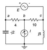
Once again we have a situation of a voltage source lacking a series impedance which makes a source conversion impossible. Without having to short it and thus treating nodes \(a\) and \(c\) as an explicit supernode, we can take an alternate route. We begin by noting that the currents entering and exiting the voltage source must be identical.
The circuit is redrawn in Figure \(\PageIndex{18}\) with the nodes and convenient current directions labeled. The circuit also uses equivalent conductances and susceptances in place of the original resistances and reactances in order to speed the process of simplifying the equations. Unlike the basic supernode technique, this time the voltage source is left in.
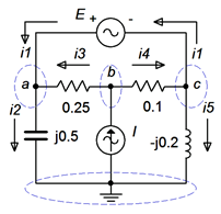
The key observation is that \(v_c = v_a − 20 \angle 0^{\circ}\) V. In other words, \(v_c\) is locked to \(v_a\) and if we find one of them, we can determine the other. Therefore, instead of writing three equations using three unknowns, we shall instead refer to node \(c\) in reference to node \(a\). In other words, wherever we need \(v_c\) we instead shall write \(v_a − 20 \angle 0^{\circ}\) V. Thus, this three node circuit will only need two equations.
We begin at node \(a\) and apply KCL as usual.
\[\sum i_{in} = \sum i_{out} \nonumber \]
\[i_1 + i_3 = i_2 \nonumber \]
This is expanded using Ohm's law and we solve for \(i_1\):
\[i_1 = i_2 −i_3 \nonumber \]
\[i_1 = j 0.5Sv_a −0.25S(v_b −v_a ) \nonumber \]
\[i_1 = (0.25 +j 0.5)Sv_a −0.25Sv_b \nonumber \]
On to node \(b\):
\[I = i_3+i_4 \nonumber \]
\[2 \angle 45^{\circ} A = 0.25S(v_b −v_a ) +0.1S(v_b −v_c ) \nonumber \]
\[2 \angle 45^{\circ} A = 0.25S(v_b −v_a ) +0.1S(v_b −(v_a −20 \angle 0^{\circ} V)) \nonumber \]
\[2 \angle 45^{\circ} A = 0.25S(v_b −v_a ) +0.1S(v_b −v_a +20 \angle 0^{\circ} V) \nonumber \]
\[2 \angle 45^{\circ} A = 0.25S(v_b −v_a ) +0.1S(v_b −v_a ) +2 \angle 0^{\circ} A \nonumber \]
\[1.531 \angle 112.5^{\circ} A =−0.35Sv_a +0.35Sv_b \nonumber \]
And finally node \(c\):
\[i_4 = i_1 +i_5 \nonumber \]
\[i_1 = i_4 −i_5 \nonumber \]
\[i_1 = 0.1S(v_b −v_c )−(− j 0.2S)v_c \nonumber \]
\[i_1 = 0.1S(v_b −(v_a−20 \angle 0^{\circ} V)) +j 0.2S(v_a −20 \angle 0^{\circ} V) \nonumber \]
\[i_1 = 0.1S(v_b −v_a +20 \angle 0^{\circ} V) +j0.2S(v_a −20 \angle 0^{\circ} V) \nonumber \]
\[i_1 = 0.1S(v_b −v_a ) +j 0.2Sv_a +(2 − j 4)A \nonumber \]
\[i_1 = (−0.1 +j 0.2)Sv_a +0.1Sv_b +4.472 \angle −63.4^{\circ} A \nonumber \]
The equations for nodes \(a\) and \(c\) both equal \(i_1\), thus they equal each other.
\[(0.25+j 0.5)Sv_a −0.25Sv_b = (−0.1 +j 0.2)Sv_a +0.1Sv_b +4.472 \angle −63.4^{\circ} A 4.472 \angle −63.4^{\circ} A = (0.35 +j 0.3)Sv_a − 0.35Sv_b \nonumber \]
The final equations are:
\[4.472 \angle −63.4^{\circ} A = (0.35 +j 0.3)Sv_a − 0.35Sv_b \nonumber \]
\[1.531 \angle 112.5^{\circ} A =−0.35Sv_a +0.35Sv_b \nonumber \]
The solution is \(v_a = 9.823 \angle -151.3^{\circ}\) volts and \(v_b = 10.31 \angle -176.2^{\circ}\) volts. As \(v_c\) is \(20 \angle 0^{\circ}\) volts less than \(v_a\), then \(v_c = 29 \angle -170.6^{\circ}\) volts. KCL summations at each of the three nodes will verify these values.