
8.2: Series Resonance
- Page ID
- 25287

\( \newcommand{\vecs}[1]{\overset { \scriptstyle \rightharpoonup} {\mathbf{#1}} } \)
\( \newcommand{\vecd}[1]{\overset{-\!-\!\rightharpoonup}{\vphantom{a}\smash {#1}}} \)
\( \newcommand{\id}{\mathrm{id}}\) \( \newcommand{\Span}{\mathrm{span}}\)
( \newcommand{\kernel}{\mathrm{null}\,}\) \( \newcommand{\range}{\mathrm{range}\,}\)
\( \newcommand{\RealPart}{\mathrm{Re}}\) \( \newcommand{\ImaginaryPart}{\mathrm{Im}}\)
\( \newcommand{\Argument}{\mathrm{Arg}}\) \( \newcommand{\norm}[1]{\| #1 \|}\)
\( \newcommand{\inner}[2]{\langle #1, #2 \rangle}\)
\( \newcommand{\Span}{\mathrm{span}}\)
\( \newcommand{\id}{\mathrm{id}}\)
\( \newcommand{\Span}{\mathrm{span}}\)
\( \newcommand{\kernel}{\mathrm{null}\,}\)
\( \newcommand{\range}{\mathrm{range}\,}\)
\( \newcommand{\RealPart}{\mathrm{Re}}\)
\( \newcommand{\ImaginaryPart}{\mathrm{Im}}\)
\( \newcommand{\Argument}{\mathrm{Arg}}\)
\( \newcommand{\norm}[1]{\| #1 \|}\)
\( \newcommand{\inner}[2]{\langle #1, #2 \rangle}\)
\( \newcommand{\Span}{\mathrm{span}}\) \( \newcommand{\AA}{\unicode[.8,0]{x212B}}\)
\( \newcommand{\vectorA}[1]{\vec{#1}} % arrow\)
\( \newcommand{\vectorAt}[1]{\vec{\text{#1}}} % arrow\)
\( \newcommand{\vectorB}[1]{\overset { \scriptstyle \rightharpoonup} {\mathbf{#1}} } \)
\( \newcommand{\vectorC}[1]{\textbf{#1}} \)
\( \newcommand{\vectorD}[1]{\overrightarrow{#1}} \)
\( \newcommand{\vectorDt}[1]{\overrightarrow{\text{#1}}} \)
\( \newcommand{\vectE}[1]{\overset{-\!-\!\rightharpoonup}{\vphantom{a}\smash{\mathbf {#1}}}} \)
\( \newcommand{\vecs}[1]{\overset { \scriptstyle \rightharpoonup} {\mathbf{#1}} } \)
\( \newcommand{\vecd}[1]{\overset{-\!-\!\rightharpoonup}{\vphantom{a}\smash {#1}}} \)
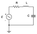
\(\newcommand{\avec}{\mathbf a}\) \(\newcommand{\bvec}{\mathbf b}\) \(\newcommand{\cvec}{\mathbf c}\) \(\newcommand{\dvec}{\mathbf d}\) \(\newcommand{\dtil}{\widetilde{\mathbf d}}\) \(\newcommand{\evec}{\mathbf e}\) \(\newcommand{\fvec}{\mathbf f}\) \(\newcommand{\nvec}{\mathbf n}\) \(\newcommand{\pvec}{\mathbf p}\) \(\newcommand{\qvec}{\mathbf q}\) \(\newcommand{\svec}{\mathbf s}\) \(\newcommand{\tvec}{\mathbf t}\) \(\newcommand{\uvec}{\mathbf u}\) \(\newcommand{\vvec}{\mathbf v}\) \(\newcommand{\wvec}{\mathbf w}\) \(\newcommand{\xvec}{\mathbf x}\) \(\newcommand{\yvec}{\mathbf y}\) \(\newcommand{\zvec}{\mathbf z}\) \(\newcommand{\rvec}{\mathbf r}\) \(\newcommand{\mvec}{\mathbf m}\) \(\newcommand{\zerovec}{\mathbf 0}\) \(\newcommand{\onevec}{\mathbf 1}\) \(\newcommand{\real}{\mathbb R}\) \(\newcommand{\twovec}[2]{\left[\begin{array}{r}#1 \\ #2 \end{array}\right]}\) \(\newcommand{\ctwovec}[2]{\left[\begin{array}{c}#1 \\ #2 \end{array}\right]}\) \(\newcommand{\threevec}[3]{\left[\begin{array}{r}#1 \\ #2 \\ #3 \end{array}\right]}\) \(\newcommand{\cthreevec}[3]{\left[\begin{array}{c}#1 \\ #2 \\ #3 \end{array}\right]}\) \(\newcommand{\fourvec}[4]{\left[\begin{array}{r}#1 \\ #2 \\ #3 \\ #4 \end{array}\right]}\) \(\newcommand{\cfourvec}[4]{\left[\begin{array}{c}#1 \\ #2 \\ #3 \\ #4 \end{array}\right]}\) \(\newcommand{\fivevec}[5]{\left[\begin{array}{r}#1 \\ #2 \\ #3 \\ #4 \\ #5 \\ \end{array}\right]}\) \(\newcommand{\cfivevec}[5]{\left[\begin{array}{c}#1 \\ #2 \\ #3 \\ #4 \\ #5 \\ \end{array}\right]}\) \(\newcommand{\mattwo}[4]{\left[\begin{array}{rr}#1 \amp #2 \\ #3 \amp #4 \\ \end{array}\right]}\) \(\newcommand{\laspan}[1]{\text{Span}\{#1\}}\) \(\newcommand{\bcal}{\cal B}\) \(\newcommand{\ccal}{\cal C}\) \(\newcommand{\scal}{\cal S}\) \(\newcommand{\wcal}{\cal W}\) \(\newcommand{\ecal}{\cal E}\) \(\newcommand{\coords}[2]{\left\{#1\right\}_{#2}}\) \(\newcommand{\gray}[1]{\color{gray}{#1}}\) \(\newcommand{\lgray}[1]{\color{lightgray}{#1}}\) \(\newcommand{\rank}{\operatorname{rank}}\) \(\newcommand{\row}{\text{Row}}\) \(\newcommand{\col}{\text{Col}}\) \(\renewcommand{\row}{\text{Row}}\) \(\newcommand{\nul}{\text{Nul}}\) \(\newcommand{\var}{\text{Var}}\) \(\newcommand{\corr}{\text{corr}}\) \(\newcommand{\len}[1]{\left|#1\right|}\) \(\newcommand{\bbar}{\overline{\bvec}}\) \(\newcommand{\bhat}{\widehat{\bvec}}\) \(\newcommand{\bperp}{\bvec^\perp}\) \(\newcommand{\xhat}{\widehat{\xvec}}\) \(\newcommand{\vhat}{\widehat{\vvec}}\) \(\newcommand{\uhat}{\widehat{\uvec}}\) \(\newcommand{\what}{\widehat{\wvec}}\) \(\newcommand{\Sighat}{\widehat{\Sigma}}\) \(\newcommand{\lt}{<}\) \(\newcommand{\gt}{>}\) \(\newcommand{\amp}{&}\) \(\definecolor{fillinmathshade}{gray}{0.9}\)Let's begin with the simplest RLC circuit; one consisting of a single voltage source in series with a single resistor, inductor and capacitor, as shown in Figure \(\PageIndex{1}\). Of particular interest is how the total impedance varies across the frequency spectrum and what impact this has on the current and the three component voltages.
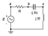
The impedance as seen by the source is simply the sum of the three components, or
\[Z = R+ jX_L − j X_C \nonumber \]
This can be expanded into
\[Z = = R+ j 2\pi f L −j \frac{1}{2\pi f C} \nonumber \]
The interesting part here is that the first term is not a function of frequency, the second term is directly proportional to frequency and the third is inversely proportional to frequency. Further, given that the positive and negative reactances behave oppositely, it appears that at some frequency they may cancel out, leaving just the resistance.
To refine this, we expect that at low frequencies the capacitor will dominate the impedance. In other words, \(X_C\) will be the largest of the three ohmic values. This means that the overall impedance will tend to mimic both the magnitude and phase of the capacitive reactance. On the other hand, at very high frequencies the inductor will tend to dominate the impedance. \(X_L\) will be the largest of the three values. In this region, the combined impedance will echo that of the inductor. In short, at low frequencies the impedance magnitude will be large and the circuit will appear capacitive while at high frequencies the impedance magnitude will be large and the circuit will appear inductive. In the middle is where things get interesting.
A plot of the resistance or reactance of the three elements is shown in Figure \(\PageIndex{2}\). The sum of the three is also shown (red). The frequency axis is uses a logarithmic scale to show the symmetrical nature of the combined impedance curve.
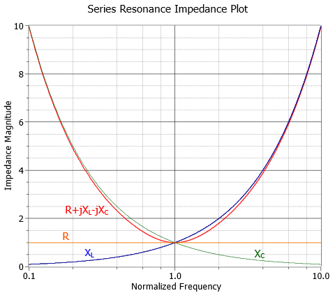
The dip in the center corresponds to an impedance equal to \(R\). At this frequency the capacitive and inductive reactances are equal in magnitude and effectively cancel each other. All that's left is the resistive component, \(R\). This frequency is known as the resonant frequency and is denoted by \(f_0\).
\[\text{The series resonant frequency, } f_0, \text{ is the frequency at which the magnitudes of the inductive and capacitive reactances are equal.} \label{8.1} \]
This implies that the power factor is unity at resonance. Also, in a real world circuit \(R\) is the combination of the series resistance plus any resistance from the inductor's coil. We can derive a formula for \(f_0\) as follows. The definition declares that the magnitude of \(X_L\) must equal the magnitude of \(X_C\). Therefore, we can set the capacitive and inductive reactance formulas equal to each other and then solve for the resulting frequency.
\[X_C = \frac{1}{2\pi f C} \\ X_L = 2\pi f L \\ X_L = X_C \\ 2\pi f_0 L = \frac{1}{2\pi f_0C} \\ f_0^2 = \frac{1}{(2\pi )^2 LC} \\ f_0 = \frac{1}{2\pi \sqrt{LC}} \label{8.2} \]
Note that a particular resonant frequency can be obtained through a variety of LC pairs. This, along with the value of \(R\), will alter the specific shape of the impedance curve in terms of how narrow or broad the dip is. These components will also affect how quickly the phase response shifts from fully capacitive (\(−90^{\circ}\)) to fully inductive (\(+90^{\circ}\)). This shape factor is described by the parameter, \(Q\). The tighter or more narrow the curve, the higher the \(Q\).
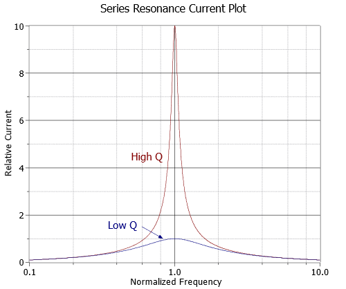
Given a constant voltage source, it should be no surprise that a plot of the resulting current will be an inversion of the impedance curve. This is shown in Figure \(\PageIndex{3}\).
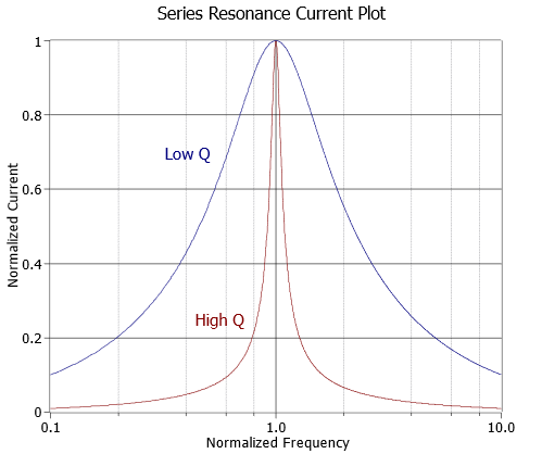
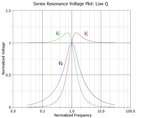
If we scale the curves such that they both have a normalized peak of unity, the difference in the shapes may be a little easier to see. This is shown in Figure \(\PageIndex{4}\).
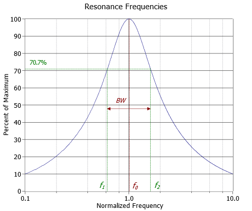
At this point we can more precisely define \(Q\). Specifically, the “sharpness” of the curve is related to the half-power or “−3 dB” frequencies, \(f_1\) and \(f_2\).1 These are the frequencies at which the current (assuming voltage source drive) falls off to 0.707 of the maximum value at resonance. Therefore, they represent the frequencies at which power will have fallen to one-half of the maximum value seen at resonance (recall that power varies as the square of current and that 0.707 squared is approximately 0.5). \(f_1\) is below \(f_0\) and \(f_2\) is found above. The difference between these two frequencies is called the bandwidth, BW.
\[BW = f_2 − f_1 \label{8.3} \]
\[Q_{circuit} = \frac{f_0}{BW} \label{8.4} \]
The relationship between these variables is illustrated in Figure \(\PageIndex{5}\). The vertical axis is shown as a percentage of maximum. For a series resonant circuit driven by a voltage source, this axis is current; however, it can be voltage in the the case of a parallel resonant circuit, as we shall see. If this plot is compared to the curves in Figure \(\PageIndex{4}\), it should be apparent that for lower \(Q\) circuits, \(f_1\) and \(f_2\) spread apart, moving away from the resonant frequency, \(f_0\). Thus, for any given \(f_0\), a lower \(Q\) means a wider (larger) bandwidth.
The resonant frequency, \(f_0\), in general is not located evenly between \(f_1\) and \(f_2\). It is, in fact, located at their geometric mean. In other words,
\[f_0 = \sqrt{f_1 f_2} \label{8.5} \]
From Equation \ref{8.5} we may derive:
\[\frac{f_0}{f_1} = \frac{f_2}{f_0} \label{8.6} \]
To find accurate values for \(f_1\) and \(f_2\) we can define a factor, \(k_0\). The derivation of \(k_0\) is found in Appendix C.
\[k_0 = \frac{1}{2Q_{circuit}} + \sqrt{\frac{1}{4{Q_{circuit}}^2} +1} \label{8.7} \]
\[f_1 = \frac{f_0}{k_0} \label{8.8} \]
\[f_2 = f_0\times k_0 \label{8.9} \]
For higher \(Q\) circuits (\(Q_{circuit} \geq 10\)), we can approximate symmetry, and thus
\[f_1 \approx f_0 − \frac{BW}{2} \label{8.10} \]
\[f_2 \approx f_0+ \frac{BW}{2} \label{8.11} \]
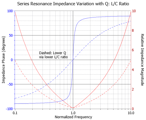
As mentioned previously, the \(Q\) can be a function of either \(R\) or the \(L/C\) ratio. In Figures \(\PageIndex{6}\) and \(\PageIndex{7}\) we have impedance curves for the two cases. The frequency axis is normalized to \(f_0\) (i.e., \(f_0\) is unity). In Figure \(\PageIndex{6}\) we vary the resistance value to see how it affects both the magnitude and phase of the impedance across frequency. Figure \(\PageIndex{7}\) is similar except we vary the inductor/capacitor ratio.
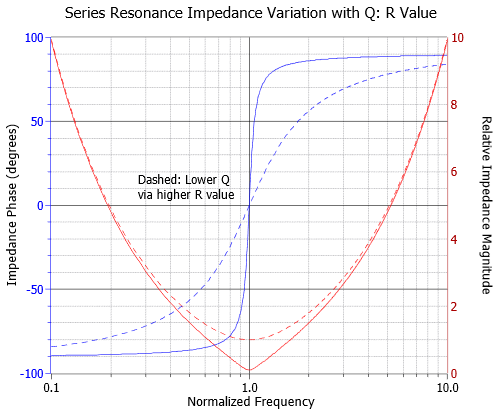
Looking first at the phase (blue, left axis), we see in both cases that high \(Q\) circuits exhibit a quick transition from a negative (capacitive) phase angle to a positive (inductive) phase angle. We also notice that the phase shift hits zero at \(f_0\), implying unity power factor.
The impedance magnitude plots show a slightly different story. While it is true that the higher \(Q\) plots are sharper, they get that way through different mechanisms. In the case of the resistor, a lower \(Q\) is achieved via a larger resistance. This has the effect of blunting the tip of the curve and lowering current flow at \(f_0\) when compared to the high \(Q\) case (as seen in Figure \(\PageIndex{3}\)). In contrast, reducing \(Q\) by reducing the inductor/capacitor ratio broadens the entire curve. The impedance magnitude at the dip does not change, and thus the current at \(f_0\) does not change. In practical terms, the \(Q\) for a series circuit, \(Q_{series}\), may also be defined by the ratio of circuit reactance to the total series resistance at resonance.
\[Q_{series} = \frac{X_0}{R_T} \label{8.12} \]
Where
\(Q_{series}\) is the \(Q\) of the series resonant circuit (i.e., \(Q_{circuit}\) for series),
\(R_T\) is the total series resistance (\(R_{series} + R_{coil}\)),
\(X_0\) is the reactance (either \(X_L\) or \(X_C\)) at \(f_0\).
From Equation \ref{8.12} we can derive an expression for \(Q_{series}\) in terms of \(R\), \(L\) and \(C\) as follows:
\[Q_{series} = \frac{X_0}{R_T} \nonumber \]
\[Q_{series} = \frac{\sqrt{X_0^2}}{R_T} \nonumber \]
At resonance \(X_L\) and \(X_C\) have the same magnitude, thus we can also say:
\[Q_{series} = \frac{\sqrt{X_L X_C}}{R_T} \nonumber \]
\[Q_{series} = \frac{1}{R_T} \sqrt{X_L X_C} \nonumber \]
\[Q_{series} = \frac{1}{R_T} \sqrt{ \frac{2 \pi f L}{2\pi f C}} \nonumber \]
Which simplifies to:
\[Q_{series} = \frac{1}{R_T} \sqrt{\frac{L}{C}} \label{8.13} \]
Effect of Q on Component Voltages
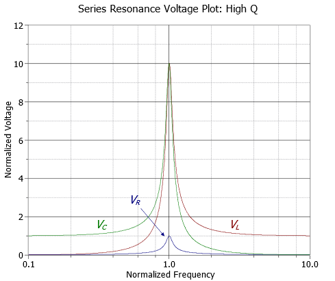
\(Q\) will create a multiplying effect on the inductor and capacitor voltages at resonance. At \(f_0\), the current through the circuit will equal the source voltage divided by \(R\) because \(X_C\) and \(X_L\) cancel. This current is also flowing through the capacitor and inductor. Equation \ref{8.12} shows that their reactances are \(Q\) times higher than \(R\), and therefore their voltages will be \(Q\) times higher than the source voltage. KVL is not violated because the voltages across \(L\) and \(C\) are 180 degrees out of phase and cancel each other. As the circuit \(Q\) is increased, the voltage multiplying effect becomes more pronounced. In extreme cases it is possible to produce inductor and capacitor voltages that are more than 100 times larger than the source voltage. As we move away from the resonant frequency, the multiplying effect decreases. At frequencies much lower than \(f_0\), almost all of the source voltage will appear across the capacitor with little for the resistor and inductor. At much higher frequencies, nearly all of the source potential appears across the inductor with nothing seen across the capacitor or resistor. This can be seen in Figure \(\PageIndex{8}\), where the source voltage is unity.
As \(Q\) decreases, not only do the capacitor and inductor voltages decrease, but another effect comes into play. At relatively high \(Q\) values, say 10 or more, the capacitor and inductor maximum voltages occur at approximately \(f_0\). At lower \(Q\) values the peaks tend to spread apart, with the capacitor's peak below \(f_0\) and that of the inductor above \(f_0\). This is illustrated in Figure \(\PageIndex{9}\) (again, the source is unity).
Example \(\PageIndex{1}\)
Consider the series circuit of Figure \(\PageIndex{10}\) with the following parameters: the source is 10 volts peak, \(L\) = 1 mH, \(C\) = 1 nF and \(R = 50 \Omega \). Find the resonant frequency, the system \(Q\) and bandwidth, and the half-power frequencies \(f_1\) and \(f_2\).
We begin by finding the resonant frequency.
\[f_0 = \frac{1}{2\pi \sqrt{LC}} \nonumber \]
\[f_0 = \frac{1}{2\pi \sqrt{1e-3\cdot 1e-9}} \nonumber \]
\[f_0 = 159 kHz \nonumber \]
We now find the magnitude of the inductive reactance, and from that, the system \(Q_{series}\) via Equation \ref{8.12}.
\[X_L = 2\pi f_0 L \nonumber \]
\[X_L = 2\pi 159 kHz 1mH \nonumber \]
\[X_L = 1000\Omega \nonumber \]
\[Q_{series} = \frac{X_L}{R_T} \nonumber \]
\[Q_{series} = \frac{1000\Omega}{50\Omega} \nonumber \]
\[Q_{series} = 20 \nonumber \]
Knowing the \(Q\), the bandwidth and corner frequencies can be found via Equations \ref{8.4}, \ref{8.10} and \ref{8.11}.
\[BW = \frac{f_0}{Q} \nonumber \]
\[BW = \frac{159 kHz}{20} \nonumber \]
\[BW = 7.95 kHz \nonumber \]
\[f_1 = f_0 − \frac{BW}{2} \nonumber \]
\[f_1 = 159 kHz − \frac{7.95kHz}{2} \nonumber \]
\[f_1 \approx 155 kHz \nonumber \]
\[f_2 = f_0 + \frac{BW}{2} \nonumber \]
\[f_2 = 159 kHz + \frac{7.95kHz}{2} \nonumber \]
\[f_2 \approx 163 kHz \nonumber \]
Given the 10 volt peak source, the voltages across the capacitor and inductor at the resonance frequency of 159 kHz would be \(Q\) times greater, or 200 volts. At higher or lower frequencies, the increased impedance lowers the current and also lowers the voltages across the components. At low frequencies, most of the source will appear across the capacitor while at high frequencies the inductor voltage will approach the source voltage.
Refining Series Q
As noted in Chapter 2, all inductors have some series resistance associated with them, usually called \(R_{coil}\). This resistance needs to be included as part of the overall circuit resistance, adding to whatever other series resistance exists. While it is possible to measure the DC resistance of a coil using a DMM, this will not necessarily give an accurate value at high frequencies. Thus, a preferred method is to determine \(Q_{coil}\) at the desired frequency from the inductor's spec sheet, and using the calculated reactance at that frequency, determine the value of \(R_{coil}\). An example of such a curve is shown in Figure \(\PageIndex{11}\).
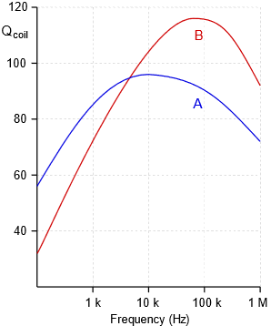
For instance, using curve A, \(Q_{coil}\) at 100 kHz is approximately 90. If \(X_L\) is 450 \(\Omega \) at this frequency, then \(R_{coil}\) would be 450 \(\Omega /90\), or 5 \(\Omega \).
Effectively, \(Q_{coil}\) sets the ceiling for the \(Q\) of the series resonant circuit, \(Q_{series}\). That is, the system \(Q\) can never be higher than the coil \(Q\). To do so would require less resistance in the loop than \(R_{coil}\), which is a practical impossibility. It is also worth noting that \(R_{coil}\) will create a deviation in the inductor voltage compared to the ideal case. This is because \(v_L\) covers the combination of the inductive reactance in series with \(R_{coil}\), thus the magnitude will be somewhat larger than expected and the angle will be less than 90 degrees. These deviations tend to be quite small unless the inductor's \(Q\) is fairly low and the remaining circuit resistance is not very much larger than \(R_{coil}\).
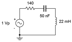
Example \(\PageIndex{2}\)
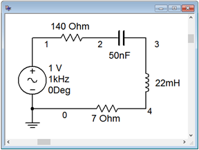
For the circuit of Figure \(\PageIndex{11}\), determine the resonant frequency, the system \(Q\), the bandwidth, and the ideal maximum voltage across each of the three components. Use curve A from Figure \(\PageIndex{11}\) for the inductor.
The first item of importance is finding the resonant frequency.
\[f_0 = \frac{1}{2 \pi \sqrt{LC}} \nonumber \]
\[f_0 = \frac{1}{2\pi \sqrt{22e-3 H50e-9F}} \nonumber \]
\[f_0 = 4.8 kHz \nonumber \]
The inductive reactance is:
\[X_L = 2\pi f_0 L \nonumber \]
\[X_L = 2\pi 4.8kHz 22 mH \nonumber \]
\[X_L = 663.3\Omega \nonumber \]
From the graph, \(Q_{coil}\) is approximately 95, meaning \(R_{coil}\) is:
\[R_{coil} = \frac{X_L}{Q_{coil}} \nonumber \]
\[R_{coil} = \frac{663.3 \Omega}{95} \nonumber \]
\[R_{coil} = 7\Omega \nonumber \]
Combined with the 140 \(\Omega \) resistor, we are left with 147 \(\Omega \), some 5% higher than if we had ignored it. The system \(Q\) is:
\[Q_{series} = \frac{X_L}{R_T} \nonumber \]
\[Q_{series} = \frac{663.3\Omega}{147\Omega} \nonumber \]
\[Q_{series} = 4.51 \nonumber \]
The \(Q\) is on the low side but not extremely so. Now for the bandwidth:
\[BW = \frac{f_0}{Q} \nonumber \]
\[BW = \frac{4.8 kHz}{4.51} \nonumber \]
\[BW = 1.06 kHz \nonumber \]
Ideally, at \(f_0\) we expect \(v_R\) will be equal to the source of 1 volt peak while the inductor and capacitor voltages will be \(Q\) times larger, or approximately 4.5 volts peak. In reality \(R_{coil}\) will create a voltage divider, reducing the drop across the 140 \(\Omega \) resistor to about 0.95 volts. The change in \(v_L\) will be negligible due to \(Z_L\) being \(663.34\angle 89.4^{\circ} \Omega \) versus the ideal \(663.3\angle 90^{\circ} \Omega \). The system \(Q\) is relatively low (\(<10\)), so the \(v_C\) and \(v_L\) peaks will shift a little from \(f_0\), with \(v_C\) peaking at a slightly lower frequency and \(v_L\) slightly higher.
Computer Simulation
Of particular interest in the prior example is the precise shape of the component responses versus frequency. This can be produced via an AC or frequency domain simulation. The circuit of Figure \(\PageIndex{12}\) is captured in a simulator as shown in Figure \(\PageIndex{13}\), and is modified by adding the inductor's coil resistance below the inductor.
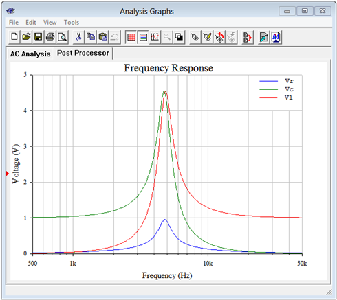
The items of interest are the net resistor voltage which appears between nodes 1 and 2, the capacitor voltage between nodes 2 and 3, and the inductor voltage which appears from node 3 to ground. The analysis is run from 500 Hz to 50 kHz giving us a factor of 10 in frequency on either side of \(f_0\), as seen in Figure \(\PageIndex{14}\). First, the peaks are just below 5 kHz, as expected. The resistor voltage (blue) is about 0.95 volts, and the inductor (red) and capacitor (green) voltages are about 4.5 volts, as calculated.
Also, note that there is a slight spread between the peaks of the capacitor and inductor voltages, with \(v_C\) slightly below \(f_0\) and \(v_L\) slightly above, again just as expected. At the lowest frequencies, all of the source appears across the capacitor while at the highest frequencies all of the source appears across the inductor. Note the similarity between these curves and those of Figures \(\PageIndex{8}\) and \(\PageIndex{9}\)
And now for a change of pace; a design problem.
Example \(\PageIndex{3}\)
Design a series resonant circuit with a resonant frequency of 100 kHz and a bandwidth of 2 kHz using a 10 mH inductor. Assumes the inductor follows curve B in Figure \(\PageIndex{14}\).
We can find the value for the capacitance by rearranging the resonance frequency equation:
\[f_0 = \frac{1}{2\pi \sqrt{LC}} \nonumber \]
\[\sqrt{LC} = \frac{1}{2\pi f_0} \nonumber \]
\[C = \frac{1}{(2\pi f_0 )^2 L} \nonumber \]
\[C = \frac{1}{(2\pi 100 kHz )^2 10mH} \nonumber \]
\[C = 253.3 pF \nonumber \]
Knowing the bandwidth and resonant frequency, we can find the system \(Q\):
\[Q_{series} = \frac{f_0}{BW} \nonumber \]
\[Q_{series} = \frac{100 kHz}{2 kHz} \nonumber \]
\[Q_{series} = 50 \nonumber \]
At resonance, the inductive reactance will be:
\[X_L = 2\pi f_0 L \nonumber \]
\[X_L = 2\pi 100 kHz 10 mH \nonumber \]
\[X_L = 6283\Omega \nonumber \]
The preceding tells us that the total series resistance must be:
\[R_{series} = \frac{X_L}{Q_{series}} \nonumber \]
\[R_{series} = \frac{6283\Omega}{50} \nonumber \]
\[R_{series} = 125.7\Omega \nonumber \]
Curve B indicates that \(Q_{coil}\) is approximately 115 at 100 kHz. Thus, \(R_{coil}\) is:
\[R_{coil} = \frac{X_L}{Q_{coil}} \nonumber \]
\[R_{coil} = \frac{6283\Omega}{115} \nonumber \]
\[R_{coil} = 54.6\Omega \nonumber \]
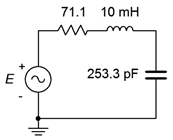
Consequently, we must add \(125.7 \Omega − 54.6 \Omega \), or \(71.1 \Omega \), to the series network to achieve the desired system \(Q\). Failure to do so will yield a much higher \(Q\) than specified, resulting in a much reduced bandwidth. The completed design is shown in Figure \(\PageIndex{15}\).
References
1Decibels are covered in detail in Chapter 10.