9.4: Power Factor Correction
- Page ID
- 25296

\( \newcommand{\vecs}[1]{\overset { \scriptstyle \rightharpoonup} {\mathbf{#1}} } \)
\( \newcommand{\vecd}[1]{\overset{-\!-\!\rightharpoonup}{\vphantom{a}\smash {#1}}} \)
\( \newcommand{\dsum}{\displaystyle\sum\limits} \)
\( \newcommand{\dint}{\displaystyle\int\limits} \)
\( \newcommand{\dlim}{\displaystyle\lim\limits} \)
\( \newcommand{\id}{\mathrm{id}}\) \( \newcommand{\Span}{\mathrm{span}}\)
( \newcommand{\kernel}{\mathrm{null}\,}\) \( \newcommand{\range}{\mathrm{range}\,}\)
\( \newcommand{\RealPart}{\mathrm{Re}}\) \( \newcommand{\ImaginaryPart}{\mathrm{Im}}\)
\( \newcommand{\Argument}{\mathrm{Arg}}\) \( \newcommand{\norm}[1]{\| #1 \|}\)
\( \newcommand{\inner}[2]{\langle #1, #2 \rangle}\)
\( \newcommand{\Span}{\mathrm{span}}\)
\( \newcommand{\id}{\mathrm{id}}\)
\( \newcommand{\Span}{\mathrm{span}}\)
\( \newcommand{\kernel}{\mathrm{null}\,}\)
\( \newcommand{\range}{\mathrm{range}\,}\)
\( \newcommand{\RealPart}{\mathrm{Re}}\)
\( \newcommand{\ImaginaryPart}{\mathrm{Im}}\)
\( \newcommand{\Argument}{\mathrm{Arg}}\)
\( \newcommand{\norm}[1]{\| #1 \|}\)
\( \newcommand{\inner}[2]{\langle #1, #2 \rangle}\)
\( \newcommand{\Span}{\mathrm{span}}\) \( \newcommand{\AA}{\unicode[.8,0]{x212B}}\)
\( \newcommand{\vectorA}[1]{\vec{#1}} % arrow\)
\( \newcommand{\vectorAt}[1]{\vec{\text{#1}}} % arrow\)
\( \newcommand{\vectorB}[1]{\overset { \scriptstyle \rightharpoonup} {\mathbf{#1}} } \)
\( \newcommand{\vectorC}[1]{\textbf{#1}} \)
\( \newcommand{\vectorD}[1]{\overrightarrow{#1}} \)
\( \newcommand{\vectorDt}[1]{\overrightarrow{\text{#1}}} \)
\( \newcommand{\vectE}[1]{\overset{-\!-\!\rightharpoonup}{\vphantom{a}\smash{\mathbf {#1}}}} \)
\( \newcommand{\vecs}[1]{\overset { \scriptstyle \rightharpoonup} {\mathbf{#1}} } \)
\(\newcommand{\longvect}{\overrightarrow}\)
\( \newcommand{\vecd}[1]{\overset{-\!-\!\rightharpoonup}{\vphantom{a}\smash {#1}}} \)
\(\newcommand{\avec}{\mathbf a}\) \(\newcommand{\bvec}{\mathbf b}\) \(\newcommand{\cvec}{\mathbf c}\) \(\newcommand{\dvec}{\mathbf d}\) \(\newcommand{\dtil}{\widetilde{\mathbf d}}\) \(\newcommand{\evec}{\mathbf e}\) \(\newcommand{\fvec}{\mathbf f}\) \(\newcommand{\nvec}{\mathbf n}\) \(\newcommand{\pvec}{\mathbf p}\) \(\newcommand{\qvec}{\mathbf q}\) \(\newcommand{\svec}{\mathbf s}\) \(\newcommand{\tvec}{\mathbf t}\) \(\newcommand{\uvec}{\mathbf u}\) \(\newcommand{\vvec}{\mathbf v}\) \(\newcommand{\wvec}{\mathbf w}\) \(\newcommand{\xvec}{\mathbf x}\) \(\newcommand{\yvec}{\mathbf y}\) \(\newcommand{\zvec}{\mathbf z}\) \(\newcommand{\rvec}{\mathbf r}\) \(\newcommand{\mvec}{\mathbf m}\) \(\newcommand{\zerovec}{\mathbf 0}\) \(\newcommand{\onevec}{\mathbf 1}\) \(\newcommand{\real}{\mathbb R}\) \(\newcommand{\twovec}[2]{\left[\begin{array}{r}#1 \\ #2 \end{array}\right]}\) \(\newcommand{\ctwovec}[2]{\left[\begin{array}{c}#1 \\ #2 \end{array}\right]}\) \(\newcommand{\threevec}[3]{\left[\begin{array}{r}#1 \\ #2 \\ #3 \end{array}\right]}\) \(\newcommand{\cthreevec}[3]{\left[\begin{array}{c}#1 \\ #2 \\ #3 \end{array}\right]}\) \(\newcommand{\fourvec}[4]{\left[\begin{array}{r}#1 \\ #2 \\ #3 \\ #4 \end{array}\right]}\) \(\newcommand{\cfourvec}[4]{\left[\begin{array}{c}#1 \\ #2 \\ #3 \\ #4 \end{array}\right]}\) \(\newcommand{\fivevec}[5]{\left[\begin{array}{r}#1 \\ #2 \\ #3 \\ #4 \\ #5 \\ \end{array}\right]}\) \(\newcommand{\cfivevec}[5]{\left[\begin{array}{c}#1 \\ #2 \\ #3 \\ #4 \\ #5 \\ \end{array}\right]}\) \(\newcommand{\mattwo}[4]{\left[\begin{array}{rr}#1 \amp #2 \\ #3 \amp #4 \\ \end{array}\right]}\) \(\newcommand{\laspan}[1]{\text{Span}\{#1\}}\) \(\newcommand{\bcal}{\cal B}\) \(\newcommand{\ccal}{\cal C}\) \(\newcommand{\scal}{\cal S}\) \(\newcommand{\wcal}{\cal W}\) \(\newcommand{\ecal}{\cal E}\) \(\newcommand{\coords}[2]{\left\{#1\right\}_{#2}}\) \(\newcommand{\gray}[1]{\color{gray}{#1}}\) \(\newcommand{\lgray}[1]{\color{lightgray}{#1}}\) \(\newcommand{\rank}{\operatorname{rank}}\) \(\newcommand{\row}{\text{Row}}\) \(\newcommand{\col}{\text{Col}}\) \(\renewcommand{\row}{\text{Row}}\) \(\newcommand{\nul}{\text{Nul}}\) \(\newcommand{\var}{\text{Var}}\) \(\newcommand{\corr}{\text{corr}}\) \(\newcommand{\len}[1]{\left|#1\right|}\) \(\newcommand{\bbar}{\overline{\bvec}}\) \(\newcommand{\bhat}{\widehat{\bvec}}\) \(\newcommand{\bperp}{\bvec^\perp}\) \(\newcommand{\xhat}{\widehat{\xvec}}\) \(\newcommand{\vhat}{\widehat{\vvec}}\) \(\newcommand{\uhat}{\widehat{\uvec}}\) \(\newcommand{\what}{\widehat{\wvec}}\) \(\newcommand{\Sighat}{\widehat{\Sigma}}\) \(\newcommand{\lt}{<}\) \(\newcommand{\gt}{>}\) \(\newcommand{\amp}{&}\) \(\definecolor{fillinmathshade}{gray}{0.9}\)As we saw in earlier work, reactive loads demand higher currents than purely resistive loads for a given true load power. The ratio between apparent power, \(S\), and true power, \(P\), is the power factor, \(PF\). Power factor may also be computed as the cosine of the load impedance angle. This situation remains for three-phase systems. If a balanced three-phase load has a large reactive component, the line current and generator phase current will be higher than necessary. The solution to this is power factor correction; the introduction of reactive elements that will counterbalance the reactive power of the load, essentially providing an opposing current such that the reactive currents cancel.
In three-phase systems the situation is potentially complicated by the fact that the load is split into three parts and can be either Y-connected or delta-connected.
The process for three phase is essentially the same as it is for single phase, but with a couple slight twists. The first course of action is to determine the reactive power, \(Q\), of the load. As we are dealing with balanced loads, it is usually easiest to just concentrate on a single leg. There are two basic possibilities. First, if the load reactance is known, it is a simple matter to determine the reactive power by finding the load phase current, squaring it, and then multiplying by the load reactance. In contrast, if the load is described in terms of a power factor, the apparent power can be computed from the generator phase voltage and current, and then the power factor can be used to find the reactive power (e.g., finding true power and then using the Pythagorean theorem). Once the reactive power is known, the required reactance can be found using power law and either the phase voltage or current. Finally, the reactance value is used to determine the component value. As many loads are inductive, the compensating component usually will be capacitive. There will three units, one for each leg of the load.
For practical purposes, the compensating device is placed across the load terminals rather than in series with it. This is true whether the load is Y-connected or delta-connected. In other words, the compensating devices always will be placed in a delta configuration. This is true even if the load is Y-connected. We shall look at both situations in the next two examples.
Example \(\PageIndex{1}\)
The Y-delta system shown in Figure \(\PageIndex{1}\) has a generator phase voltage of 120 volts RMS at 60 Hz. Determine the power factor, the generator phase current, and the total real and apparent power delivered to the load. Also determine components to correct the power factor and the new generator phase current.
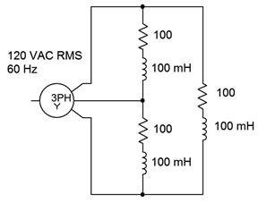
First, the power factor is the cosine of the impedance angle. At 60 Hz, the reactance of the 100 mH inductor is \(−j37.7 \Omega \). This is in series with the resistance for a load impedance of \(100 −j37.7 \Omega \) or \(106.9\angle 20.66^{\circ}\) per leg. The cosine of this angle is 0.9357.
The voltage across each leg of the load will equal the line voltage.
\[v_{line} = \sqrt{3} \times v_{phase} \nonumber \]
\[v_{line} = \sqrt{3} \times 120 V \nonumber \]
\[v_{line} \approx 207.8V RMS \nonumber \]
This will produce a load phase current magnitude of:
\[i_{load} = \frac{v_{phase}}{Z_{load}} \nonumber \]
\[i_{load} = \frac{207.8V}{106.9 \Omega} \nonumber \]
\[i_{load} \approx 1.944A RMS \nonumber \]
Now we can find the load powers.
\[S = 3\times v_{phase}\times i_{phase} \nonumber \]
\[S = 3\times 207.8V\times 1.944 A \nonumber \]
\[S \approx 1212 VA \nonumber \]
\[P = S\times PF \nonumber \]
\[P = 1212VA\times 0.9357 \nonumber \]
\[P \approx 1134 W \nonumber \]
\[Q = S \sin \theta \nonumber \]
\[Q = 1212 VA \sin 20.66^{\circ} \nonumber \]
\[Q \approx 427.6 VAR \nonumber \]
The load is inductive so the compensation components need to be capacitors. Each capacitor needs to create 427.6/3 VAR, or 142.5 VAR. The required reactance is:
\[X_C = − j \frac{{v_{phase}}^2}{Q} \nonumber \]
\[X_C = − j \frac{(207.8V)^2}{142.5VAR} \nonumber \]
\[X_C \approx − j 303 \Omega \nonumber \]
And finally, the capacitance value:
\[C = \frac{1}{2\pi f X_C} \nonumber \]
\[C = \frac{1}{2\pi 60 Hz 303 \Omega} \nonumber \]
\[C \approx 8.75\mu F \nonumber \]
These capacitors would be placed directly in parallel with each leg of the load and should result in a reduction of the generator and line currents.
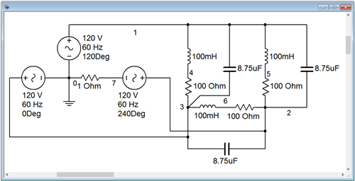
Computer Simulation
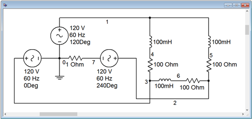
To see the effect of power factor correction, the circuit used in Example \(\PageIndex{1}\) is captured in a simulator, as illustrated in Figure \(\PageIndex{2}\). The goal here is to show the reduction in supplied current. To facilitate this, the normal Y-connected three-phase source is not used. Instead, three individual sine sources are used, each with a proper phase shift. A small 1 \( \Omega \) sensing resistor is inserted in series with one of the sources. The voltage across this resistor is easily measured (node 7) and serves as a proxy for the generator phase current. Compared to the sizes of the other components, this extra resistance will have minimal impact on overall circuit behavior, perhaps shifting current values around 1% or so. Reducing the resistance to 0.1 \( \Omega \) will reduce errors to negligible levels, but 1 \( \Omega \) is convenient as no scaling is needed and will be sufficient to show the effect of power factor correction on source current.
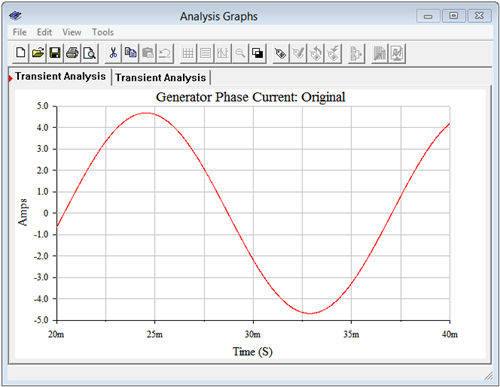
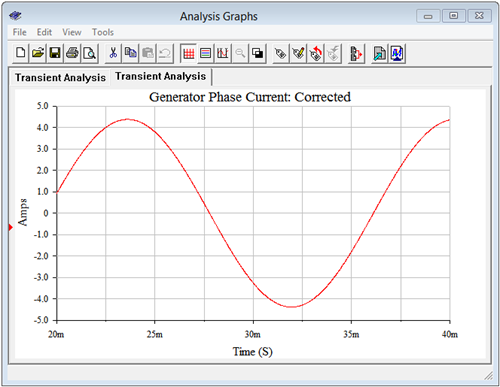
A transient simulation is run on the circuit, plotting the voltage at node 7. This is shown in Figure \(\PageIndex{3}\). Due to the 1 \( \Omega \) sensing resistance, the voltage value is the same as the current value in amps. The peak value of the current is approximately 4.7 amps. This agrees with the calculated value of 4.76 amps (1.944 amps RMS times \(\sqrt{2}\) times \(\sqrt{3}\)). Now that a baseline for the current has been established, we turn our attention to the modified version of the circuit with power factor correction.
The three power factor correction capacitors are added in parallel with the existing load legs (i.e., from line to line). This is illustrated in Figure \(\PageIndex{4}\).
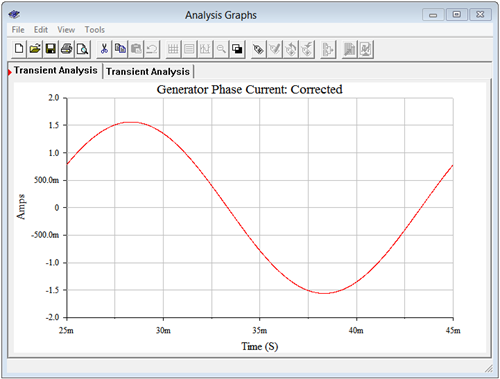
The transient simulation is repeated. The results are shown in Figure \(\PageIndex{5}\). The peak current in this version of the circuit is approximately 4.4 amps. Theoretically, the current should be scaled by the power factor, or 0.9357. As previously calculated, the value of the original generator phase current is 4.76 amps peak. Multiplying that by the power factor yields approximately 4.45 amps peak. The small deviation between this result and the simulation is due to the effect of the 1 \( \Omega \) sensing resistor.
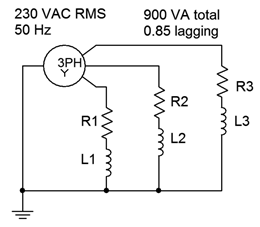
Example \(\PageIndex{2}\)
The Y-Y system shown in Figure \(\PageIndex{6}\) has a generator phase voltage of 230 volts RMS at 50 Hz. The load draws 900 VA with a power factor of 0.85 lagging. Determine the generator phase current. Also determine components to correct the power factor and the new generator phase current once the system is corrected.
We're looking for the generator phase current so let's break this down to a single leg, first. The total apparent power, \(S\), is 900 VA. For a single leg that's 300 VA. This is a Y-Y system so the generator phase current and voltage are the same as the load phase current and voltage. The current can be found via the apparent power.
\[i = \frac{S}{v} \nonumber \]
\[i = \frac{300 VA}{230 V RMS} \nonumber \]
\[i \approx 1.304A RMS \nonumber \]
Given a power factor of 0.85, we can determine the real and reactive powers.
\[P = S\times PF \nonumber \]
\[P = 300VA\times 0.85 \nonumber \]
\[P = 255W \nonumber \]
\[Q = \sqrt{S^2−P^2} \nonumber \]
\[Q = \sqrt{(300 VA)^2−(255W)^2} \nonumber \]
\[Q \approx 158 \text{ VAR inductive} \nonumber \]
For power factor correction, we need 158 VAR capacitive per leg to counteract this. These capacitors will be placed across the load terminals in a delta configuration. As such, they will see the line voltage. For a Yconnected generator, the line voltage is the phase voltage times \(\sqrt{3}\). The result here is 230 volts times \(\sqrt{3}\), or 398.4 volts RMS. From this we may determine the required reactance.
\[X_C =− j \frac{{v_{phase}}^2}{Q} \nonumber \]
\[X_C =− j \frac{(398.4V)^2}{158 VAR} \nonumber \]
\[X_C \approx − j 1004.6 \Omega \nonumber \]
The corresponding capacitance value is:
\[C = \frac{1}{2\pi f X_C} \nonumber \]
\[C = \frac{1}{2\pi 50Hz 1004.6 \Omega} \nonumber \]
\[C \approx 3.17\mu F \nonumber \]
Computer Simulation
In Example \(\PageIndex{2}\) we computed the generator phase current to be 1.304 amps RMS, which is equivalent to 1.844 amps peak. If the corrected circuit is proper, then the apparent power should fall to the real power, or 255 watts. The resulting generator phase current should be this power divided by the generator phase voltage, 255/230, or 1.109 amps RMS. This is equivalent to 1.568 amps peak. (Alternately, we could multiply the original current by the power factor because the voltage is constant.)
To verify the effectiveness of the circuit modification, we start by capturing the circuit in a simulator, as shown in Figure \(\PageIndex{7}\).
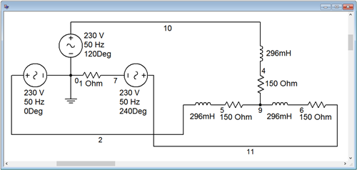
As in the prior example, the source is built from three discrete sine generators at appropriate phases. Beneath one of them, a 1 \( \Omega \) current sensing resistor is added (node 7). This value should produce no more than about 1% deviation as it is a full two orders of magnitude smaller than the other circuit resistances.
An interesting question for the sharp-eyed observer is how the load resistor and inductor values were obtained. This turns out to be not so difficult. We have already computed the true and reactive powers for each leg. We also know the load phase voltage (it's the same as the generator, 230 volts, as it's a Y-Y connection). Therefore, we can find the \(R\) and \(X_L\) values as we have already computed the load current and can use this to determine the load impedance, \(Z\). The power factor is known, and from this the real and reactive parts can be deduced.
\[Z = \frac{v_{phase}}{i} \nonumber \]
\[Z = \frac{230 V}{1.304 A} \nonumber \]
\[Z \approx 176 \Omega \nonumber \]
This is the magnitude. For the sake of completeness, the angle is the arccosine of the power factor, or \(\cos^{-1}(0.85)\), which is 31.8 degrees. The fastest way to determine \(R\) is to recognize that the real portion is the impedance magnitude times the power factor:
\[R = Z\times PF \nonumber \]
\[R = 176 \Omega \times 0.85 \nonumber \]
\[R \approx 150 \Omega \nonumber \]
The reactive portion can be found via the Pythagorean theorem or by using the power relation. Then we apply the reactance formula to find the inductance.
\[X_L = \frac{Q}{i^2} \nonumber \]
\[X_L = \frac{158VAR}{(1.304 A RMS)^2} \nonumber \]
\[X_L \approx 92.9 \Omega \nonumber \]
\[L = \frac{X_L}{2 \pi f} \nonumber \]
\[L = \frac{92.9 \Omega}{ 2\pi 50 Hz} \nonumber \]
\[L \approx 296 mH \nonumber \]
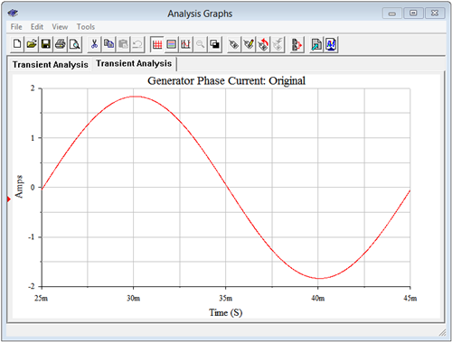
The result of a transient analysis is shown in Figure \(\PageIndex{8}\). The measured peak phase current is 1.837 amps. This compares nicely with the expected value of 1.844 amps.
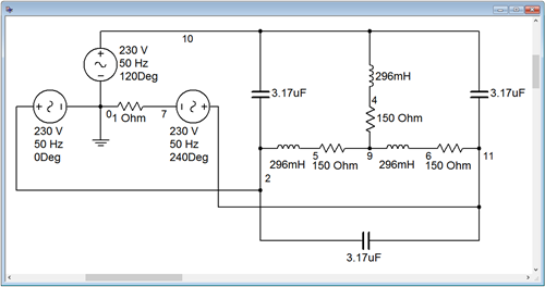
For the comparison, the power factor correction capacitors are added in a delta configuration (across the lines) as shown in Figure \(\PageIndex{9}\).
Another simulation is run, the result shown in Figure \(\PageIndex{10}\). The peak current has decreased to 1.56 amps. This is just slightly lower than the expected value of 1.568 amps peak. Again, this small deviation is due to the effect of the sense resistor.