
8.3: Parallel Resonance
- Page ID
- 25288

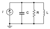
If the three RLC components are placed in parallel, as in Figure \(\PageIndex{1}\), a parallel resonant circuit can result. Typically, it would be driven by a current source as shown, although this is not a requirement for resonance. Parallel resonance is slightly more complicated than series resonance due to the fact that the series coil resistance cannot be lumped in with the remaining circuit resistance as it can with the series case. In other words, the practical reality is that we have a series-parallel circuit where the inductor is, in fact, a series combination of the inductance and the coil resistance. It turns out that usually this resistance cannot be ignored, even if it is very small. To alleviate this problem, it is possible to find a parallel equivalent for the series inductive reactance and associated coil resistance. That is, we need a series to parallel transform.
Series to Parallel Inductor Transform
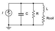
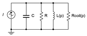
First, let's take a look at what we have in practical terms. A realistic parallel resonant circuit is illustrated in Figure \(\PageIndex{2}\). This circuit adds the internal coil resistance of the inductor to the ideal circuit shown in Figure \(\PageIndex{1}\). What we would like to do is derive a means of finding the parallel equivalent of the inductor with its coil resistance. Certainly, this should be possible to do. After all, it is a trivial exercise to do the reverse; namely, taking a parallel combination of an inductor and resistor and finding its series equivalent (i.e., expressing the resulting impedance in rectangular form). After completing the process we should have an equivalent circuit like that shown in Figure \(\PageIndex{3}\). In this equivalent circuit, \(R\) and \(C\) are the values from the original circuit while \(L_{(p)}\) and \(R_{coil(p)}\) are the parallel equivalent transformed values derived from the original inductor. In this version, it is easy to combine \(R\) in parallel with \(R_{coil(p)}\) to create a single resistor and thus wind up back at our ideal circuit of Figure \(\PageIndex{1}\).
For the equivalent transform, refer to Figure \(\PageIndex{4}\). We start with a practical coil consisting of a series combination of resistance and inductive reactance, \(R_s + jX_s\). We will find the parallel equivalent, \(R_p || jX_p\).
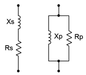
We begin with the reciprocal conductance/resistance rule:
\[R_s+jX_s = \frac{1}{\frac{1}{R_p} + \frac{1}{jX_p}} \\ \frac{1}{R_s+jX_s} = \frac{1}{R_p} + \frac{1}{jX_p} \label{8.14} \]
The next step is to isolate the real and imaginary parts of the series version. We can do this by multiplying the left term of Equation \ref{8.10} by the complex conjugate to arrive at an equivalent:
\[\frac{1}{R_s+jX_s} \frac{R_s − jX_s}{R_s − jX_s} = \frac{R_s}{R_s^2+X_s^2} + \frac{− jX_s}{R_s^2+X_s^2} \nonumber \]
Substituting this equivalent back into Equation \ref{8.14} yields,
\[\frac{R_s}{R_s^2+X_s^2} + \frac{−jX_s}{R_s^2+X_s^2} = \frac{1}{R_p} + \frac{1}{jX_p}\nonumber \]
Therefore,
\[\frac{1}{R_p} = \frac{R_s}{R_s^2+X_s^2} \nonumber \]
\[\frac{1}{jX_p} = \frac{− jX_s}{R_s^2+X_s^2} \nonumber \]
Taking the reciprocal results in:
\[R_p = \frac{R_s^2+X_s^2}{R_s} \label{8.15} \]
\[jX_p = j\frac{R_s^2+X_s^2}{X_s} \label{8.16} \]
For high \(Q\) coils (\(Q_{coil} \geq 10\)), \(X_s \gg R_s\), so we can approximate these as:
\[R_p \approx \frac{X_s^2}{R_s} = Q_{coil} X_s = Q_{coil}^2 R_s \label{8.17} \]
\[jX_p \approx j \frac{X_s^2}{X_s} = jX_s \label{8.18} \]
Thus, for a high \(Q_{coil}\), the parallel equivalent reactance is unchanged from the series value and the parallel equivalent resistance is the series resistance times the \(Q\) of the coil squared. Interestingly, Equation \ref{8.17} shows that a smaller \(R_S\) (which yields a proportionally larger \(Q_{coil}\)) results in a larger \(R_P\). Thus, the ideal inductor which would have no coil resistance results in an \(R_p\) of infinity. Due to this resistive “inversion” of the series-parallel transform, parallel circuit \(Q\) is defined as:
\[Q_{parallel} = \frac{R_T}{X_L} \label{8.19} \]
Where
\(Q_{parallel}\) is the \(Q\) of the parallel resonant circuit (i.e., \(Q_{circuit}\) for parallel),
\(R_T\) is the total parallel resistance \((R_p || R)\),
\(X_L\) is the reactance at \(f_0\).
Based on Equation \ref{8.19} and the development of Equation \ref{8.13}, it can be shown that:
\[Q_{parallel} = R_T \sqrt{C}{L} \label{8.20} \]
For higher \(Q\) circuits (\(Q_{parallel} \geq 10\)), \(f_0\) is found as in the series case (repeating):
\[f_0= \frac{1}{2 \pi \sqrt{LC}} \label{8.2} \]
For lower \(Q\) circuits, \(f_0\) will be reduced slightly due to the fact that the transformed resistance is frequency dependent. More on this in an upcoming section.
Parallel Resonance Impedance
A parallel impedance plot is shown in Figure \(\PageIndex{5}\). The effect is the inverse of the series case. At low frequencies the small inductive reactance results in a low impedance magnitude with a positive (inductive) phase angle. At high frequencies the small capacitive reactance results in a low impedance magnitude with a negative (capacitive) phase angle. At resonance the reactive values cancel. This leaves just the parallel resistive value which produces the characteristic peak in impedance. The phase angle is zero, corresponding to a power factor of unity.
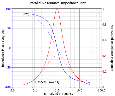
If the parallel resonant circuit is driven by a current source, then the voltage produced across the resonant circuit (sometimes referred to as a tank circuit) will echo the shape of the impedance magnitude. In other words, it will effectively discriminate against high and low frequencies and keep only those signals in the vicinity of the resonant frequency. This is one method of making a bandpass filter. The lower and upper half-power frequencies, \(f_1\) and \(f_2\), are found in the same manner as in series resonance.
Repeating for convenience:
\[BW = f_2 − f_1 \label{8.3} \]
\[Q_{circuit} = \frac{f_0}{BW} \label{8.4} \]
\[f_0 = \sqrt{f_1 f_2} \label{8.5} \]
\[\frac{f_0}{f_1} = \frac{f_2}{f_0} \label{8.6} \]
\[k_0 = \frac{1}{2Q_{circuit}} +\sqrt{\frac{1}{4{Q_{circuit}}^2} +1} \label{8.7} \]
\[f_1 = \frac{f_0}{k_0} \label{8.8} \]
\[f_2 = f_0\times k_0 \label{8.9} \]
For higher \(Q\) circuits (\(Q_{circuit} \geq 10\)), we can approximate symmetry, and thus
\[f_1 \approx f_0 − \frac{BW}{2} \label{8.10} \]
\[f_2 \approx f_0+ \frac{BW}{2} \label{8.11} \]
Finally, it is worth repeating that for relatively low \(Q\) values there will be some shifting of the resonant and half-power frequencies from the equations presented above.
There are some similarities between parallel and series resonance. Like series, as the parallel \(Q\) increases, the impedance curve becomes sharper and the phase change is more abrupt. Further, we also see an apparent “\(Q\) amplification” effect in parallel resonant circuits, however, here it will be the reactive currents that will be increased relative to the source current instead of the series component voltages.
Note that the parallel resistor can be used to lower the system \(Q\) and thus broaden the bandwidth, however, the system \(Q\) can never be higher than the \(Q\) of the inductor itself. The inductor sets the upper limit on system \(Q\) and therefore, how tight the bandwidth can be. In other words, \(Q_{circuit} \leq Q_{coil}\). This is the same situation we saw for series resonance.
Example \(\PageIndex{1}\)
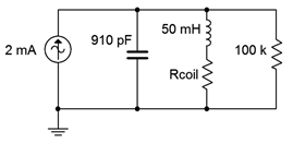
For the circuit of Figure \(\PageIndex{6}\), determine the resonant frequency, the corner frequencies of \(f_1\) and \(f_2\), the bandwidth and the system \(Q\). Also find the circuit voltage at the resonant frequency. \(R_{coil} = 100 \Omega \).
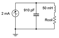
First, we'll assume this is a high \(Q (\geq 10)\) circuit.
\[f_0= \frac{1}{2\pi \sqrt{LC}} \nonumber \]
\[f_0= \frac{1}{2 \pi \sqrt{50 mH910 pF}} \nonumber \]
\[f_0=23.6 kHz \nonumber \]
\[X_L = 2\pi f L \nonumber \]
\[X_L = 2\pi 23.6kHz 50 mH \nonumber \]
\[X_L = 7.41k \Omega \nonumber \]
\[Q_{coil} = \frac{X_L}{R_{coil}} \nonumber \]
\[Q_{coil} = \frac{7.41k \Omega}{100 \Omega} \nonumber \]
\[Q_{coil} = 74.1 \nonumber \]
The parallel equivalent of the coil resistance is:
\[R_p = R_{coil} Q_{coil}^2 \nonumber \]
\[R_p = 100\Omega 74.1^2 \nonumber \]
\[R_p = 549.5 k\Omega \nonumber \]
There is no other resistor in parallel with the inductor and capacitor, therefore the equivalent parallel resistance, \(R_p\), is the total resistance of the circuit, \(R_T\). Consequently, the \(Q\) of the circuit must be the same as \(Q_{coil}\). We can verify this as follows:
\[Q_{parallel} = \frac{R_T}{X_L} \nonumber \]
\[Q_{parallel} = \frac{549.5 k \Omega}{7.41 k\Omega} \nonumber \]
\[Q_{parallel} = 74.1 \nonumber \]
Our initial assumption of high circuit \(Q\) is met.
\[BW = \frac{f_0}{Q_{parallel}} \nonumber \]
\[BW = \frac{23.6 kHz}{74.1} \nonumber \]
\[BW = 318 Hz \nonumber \]
\[f_1 \approx f_0 − \frac{BW}{2} \nonumber \]
\[f_1 \approx 23.6 kHz − \frac{318Hz}{2} \nonumber \]
\[f_1 \approx 23.44 kHz \nonumber \]
\[f_2 \approx f_0 + \frac{BW}{2} \nonumber \]
\[f_2 \approx 23.6 kHz + \frac{318 Hz}{2} \nonumber \]
\[f_2 \approx 23.76 kHz \nonumber \]
To find the circuit voltage at \(f_0\), simply multiply the resonant impedance of 549.5 k\(\Omega \) times the source of 2 mA. This yields approximately 1100 volts.
Computer Simulation
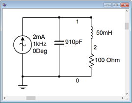
The circuit of Example \(\PageIndex{1}\) is captured in a simulator as shown in Figure \(\PageIndex{7}\).
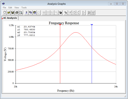
A frequency domain or AC analysis is run on the circuit, plotting the magnitude of the source voltage (node 1) from 2 kHz to 200 kHz. This will give us roughly a factor of ten on either side of the resonant frequency. The result is shown in Figure \(\PageIndex{8}\). The plot shows a clear and sharp peak in the low 20 kHz region. Note that the peak voltage is just over 1000 volts, as predicted. Figure \(\PageIndex{9}\) shows a magnified version of this plot so that we can accurately verify the peak voltage along with \(f_1\) and \(f_2\).
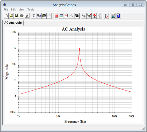
Figure \(\PageIndex{9}\) shows that the peak is indeed approximately 1100 volts. The \(f_1\) and \(f_2\) frequencies are found at 0.707 times this peak, or some 778 volts. Two measurement cursors are employed for this task. The Y values are the voltages at the cursor's intersection with the curve and the X values are the corresponding frequencies. We can see that the results are in tight agreement with the calculations. At levels of about 777 to 780 volts we obtain \(f_1\) and \(f_2\) values of approximately 23.44 kHz and 23.75 kHz, respectively.
Example \(\PageIndex{2}\)
For the circuit of Figure \(\PageIndex{10}\), determine the resonant frequency, the corner frequencies of \(f_1\) and \(f_2\), the bandwidth and the system \(Q\). Also find the circuit voltage at the resonant frequency. \(R_{coil} = 100 \Omega \).
This circuit is identical to the one in the previous example with the exception of an added 100 k\(\Omega \) load resistor. This should lower the system \(Q\) and thus widen the bandwidth. The peak impedance will also be reduced which will cause a decrease in the system voltage at resonance. Some parameters will not change. They include:
\[f_0 = 23.6 kHz \nonumber \]
\[X_L = 7.41 k \Omega \nonumber \]
\[Q_{coil} = 74.1 \nonumber \]
\[R_p = 549.5 k \Omega \nonumber \]
We'll assume this is a high \(Q (\geq 10)\) circuit.
Rp is in parallel with the load resistance of \(R\) yielding an effective parallel resistance of \(549.5 k\Omega || 100 k\Omega \), or 84.6 k\(\Omega \).
\[Q_{parallel} = \frac{R_T}{X_L} \nonumber \]
\[Q_{parallel} = \frac{84.6 k \Omega}{7.41k \Omega} \nonumber \]
\[Q_{parallel} = 11.4 \nonumber \]
The circuit \(Q\) is much reduced but our initial assumption of high circuit \(Q\) is still met. Now we can find the bandwidth and corner frequencies.
\[BW = \frac{f_0}{Q_{parallel}} \nonumber \]
\[BW = \frac{23.6 kHz}{11.4} \nonumber \]
\[BW = 2.07kHz \nonumber \]
\[f_1 \approx f_0 − \frac{BW}{2} \nonumber \]
\[f_1 \approx 23.6 kHz − \frac{2.07kHz}{2} \nonumber \]
\[f_1 \approx 22.56 kHz \nonumber \]
\[f_2 \approx f_0 + \frac{BW}{2} \nonumber \]
\[f_2 \approx 23.6 kHz + \frac{2.07kHz}{2} \nonumber \]
\[f_2 \approx 24.64 kHz \nonumber \]
The circuit voltage at \(f_0\) is reduced to 84.6 k\(\Omega \) times 2 mA, or 169.2 volts.
Computer Simulation
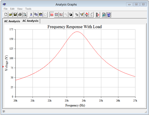
The simulation results follow those of Example \(\PageIndex{1}\) and are shown in Figure \(\PageIndex{11}\). The results agree with the computed values. The peak voltage has been reduced to about 170 volts, and \(f_1\) and \(f_2\) (found at 0.707 times the peak, or approximately 120 volts) are about 22.5 kHz and 24.6 kHz, respectively.
Example \(\PageIndex{3}\)
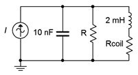
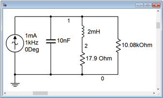
Consider the circuit of Figure \(\PageIndex{12}\) with the following parameters: \(L\) = 2 mH, \(C\) = 10 nF, and \(Q_{coil}\) = 25. Determine the resonant frequency and a value for \(R\) such that the system bandwidth is 3 kHz.
As usual, we'll assume this is a high \(Q (\geq 10)\) circuit. This is certainly true of the coil, although we have to determine the resonant frequency in order to determine the \(Q\) of the circuit.
\[f_0 = \frac{1}{2\pi \sqrt{ LC}} \nonumber \]
\[f_0 = \frac{1}{2\pi \sqrt{2mH 10 nF}} \nonumber \]
\[f_0 = 35.59 kHz \nonumber \]
\[Q_{parallel} = \frac{f_0}{BW} \nonumber \]
\[Q_{parallel} = \frac{35.59 kHz}{3 kHz} \nonumber \]
\[Q_{parallel} = 11.86 \nonumber \]
We have high \(Q\) and can continue1. Ultimately, we need to determine the total parallel resistance required to achieve this \(Q\). Before we can do that we need to determine \(X_L\).
\[X_L = 2\pi f L \nonumber \]
\[X_L = 2\pi 35.59 kHz 2mH \nonumber \]
\[X_L = 447 \Omega \nonumber \]
\[R_T = Q_{parallel} \times X_L \nonumber \]
\[R_T = 11.86\times 447\Omega \nonumber \]
\[R_T = 5.3k \Omega \nonumber \]
\(R_T\) is the parallel combination of \(R\) and \(R_p\) (the parallel equivalent of \(R_{coil}\)), so first we need to find \(R_{coil}\).
\[R_{coil} = \frac{X_L}{Q_{coil}} \nonumber \]
\[R_{coil} = \frac{447\Omega}{25} \nonumber \]
\[R_{coil} = 17.9\Omega \nonumber \]
The parallel equivalent resistance of \(R_{coil}\) is:
\[R_p = R_{coil} Q_{coil}^2 \nonumber \]
\[R_p = 17.9\Omega 25^2 \nonumber \]
\[R_p = 11.18 k\Omega \nonumber \]
Using the conductance rule, we can find the requisite value of \(R\).
\[R = \frac{1}{\frac{1}{R_T} − \frac{1}{R_p}} \nonumber \]
\[R = \frac{1}{\frac{1}{5.3k \Omega} − \frac{1}{11.18 k \Omega}} \nonumber \]
\[R = 10.08 k\Omega \nonumber \]
Thus, we need to use a 10.08 k\(\Omega \) resistor in order to lower the circuit \(Q\) enough to achieve a 3 kHz bandwidth. Without this resistor, the bandwidth will be less than half of what is required.
Computer Simulation
Figure \(\PageIndex{13}\) shows the completed design of the previous example captured in a simulator. A 1 mA current source is used for convenience of calculation.
Given that \(R_T\) is 5.3 k\(\Omega \), the 1 mA current source should produce 5.3 volts at the resonance frequency of 35.59 kHz. The results of an AC analysis are shown in Figure \(\PageIndex{14}\).
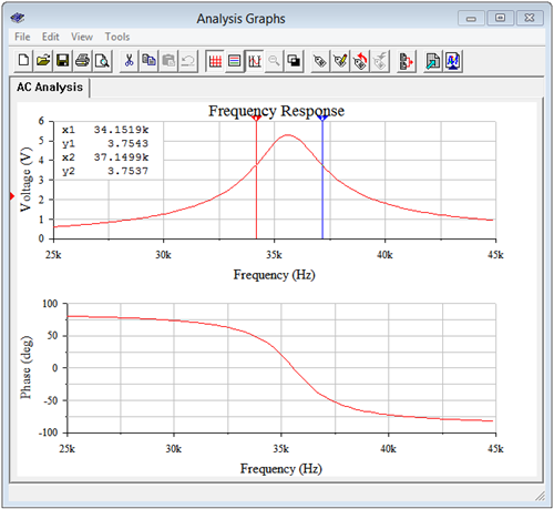
First off, the \(f_0\) of approximately 35.6 kHz is verified by both the peak in voltage and the phase angle reaching \(0^{\circ}\) at this frequency, the latter indicating perfect cancellation between the inductor and capacitor (i.e., the circuit impedance is purely resistive and achieving unity power factor). The cursors are used to obtain accurate values for \(f_1\) and \(f_2\). These frequencies are reached at 0.707 of the peak of 5.3 volts, or about 3.75 volts. The frequencies are approximately 34.15 kHz and 37.15 kHz, achieving the desired bandwidth of 3 kHz.
Low Q Parallel Resonance
There are some changes in the computations when \(Q_{parallel}\) is low. Generally, this means values below 10, although we might think of values between 5 and 10 to be a transition region where deviations of two percentage points or less come into play. Once the circuit \(Q\) falls below 5, the deviations from the high \(Q\) equations grow rapidly and quickly rise into double digit percentages. The main item of interest here is the shift in \(f_0\).
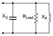
These deviations are caused by the fact that the approximations used for Equations \ref{8.17} and \ref{8.18} are no longer true. That is, with low \(Q_{coil}\) values, we can no longer assume that the transformed \(X_L\) is the same as the original \(X_L\) (i.e., \(X_p\) and \(X_s\) in Figure \(\PageIndex{4}\)). Given this fact, we can revisit the basic parallel RLC circuit, but this time using the exact value from the series-to-parallel inductor transform. This is shown in Figure \(\PageIndex{15}\). \(R_{Load}\) is the combined resistance of the parallel network while \(X_p\) is the equivalent value obtained from Equation \ref{8.16} (slightly modified and repeated for convenience):
\[X_p = \frac{X^2+R^2}{X} \nonumber \]
\(X\) and \(R\) in this equation are the original series values for the inductor. At \(f_0\), the magnitudes of the reactances are equal, or \(X_C = X_p\), therefore,
\[X_C = \frac{X^2+R^2}{X} \nonumber \]
Expanding yields:
\[\frac{1}{2\pi f_0C} = \frac{(2\pi f_0 L)^2+R^2}{2\pi f_0 L} \nonumber \]
Now rearrange and simplify.
\[\frac{2 \pi f_0 L}{2\pi f_0C} = (2\pi f_0 L)^2+R^2 \nonumber \]
\[\frac{L}{C} = (2\pi f_0 L)^2+R^2 \nonumber \]
\[(2\pi f_0 L)^2 = \frac{L}{C} −R^2 \nonumber \]
\[2\pi f_0 L = \sqrt{ \frac{L}{C} −R^2} \nonumber \]
\[2\pi f_0 = \sqrt{ \frac{1}{LC} − \frac{R^2}{L^2}} \nonumber \]
\[2\pi f_0 = \frac{1}{\sqrt{ LC}} \sqrt{1 − \frac{C R^2}{L}} \nonumber \]
And finally we come to:
\[f_0 = \frac{1}{2\pi \sqrt{ LC}} \sqrt{1 − \frac{C R^2}{L}} \label{8.21} \]
If desired, we can treat the first term as the ordinary series resonant frequency and the second term as a fractional coefficient, as in:
\[f_0 = f_{series} k_p \label{8.22} \]
Where
\[k_p = \sqrt{1 − \frac{C R^2}{L}} \label{8.23} \]
Using Equation \ref{8.20}, \(k_p\) may also be expressed as:
\[k_p = \sqrt{ 1 − \frac{1}{Q^2}} \label{8.24} \]
Examining Equation \ref{8.23} might lead to some concern, namely, what happens if the second term is greater than or equal to 1? Remember, the definition we're using for resonance is the frequency at which the reactances cancel, which means the phase angle is \(0^{\circ}\) (unity power factor). If the second term is greater than or equal to 1, the phase shift will never reach \(0^{\circ}\), and by that definition, we don't really have a resonant circuit anymore.
We will explore the reality of this situation by starting with a simple high \(Q\) parallel circuit and then investigate the changes in the magnitude and phase response as the \(Q\) is decreased. We begin with the circuit of Figure \(\PageIndex{16}\).
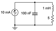
Assuming we have high circuit \(Q\), the resonant frequency is:
\[f_0= \frac{1}{2\pi \sqrt{ LC}} \nonumber \]
\[f_0= \frac{1}{2 \pi \sqrt{1 mH100 nF}} \nonumber \]
\[f_0=15.92 kHz \nonumber \]
\[X_L = 2\pi f L \nonumber \]
\[X_L = 2\pi 15.92 kHz 1mH \nonumber \]
\[X_L = 100\Omega \nonumber \]
\[Q_{coil} = \frac{X_L}{R_{coil}} \nonumber \]
\[Q_{coil} = \frac{100\Omega}{5\Omega} \nonumber \]
\[Q_{coil} = 20 \nonumber \]
There are no other resistances in the circuit, therefore \(Q_{circuit} = Q_{coil}\) and our initial assumption is correct. The circuit is captured in a simulator and an AC analysis is performed. The resulting plots are shown in Figure \(\PageIndex{17}\).
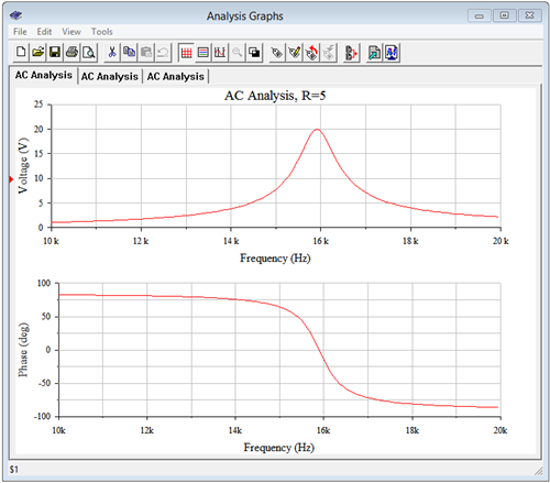
The resonant frequency appears to be just under 16 kHz, as predicted. Cursor-based measurement of the frequency at which the phase crosses \(0^{\circ}\) yields 15.89 kHz. This turns out to be even closer than it seems. In spite of the high circuit \(Q\), \(k_p\) was calculated and as expected is very close to unity, namely 0.99875. When multiplied by the ideal \(f_0\) (i.e., using Equation \ref{8.22}), we arrive at 15.90 kHz. Splitting hairs perhaps, but it's good to know the deviation is shrinking.
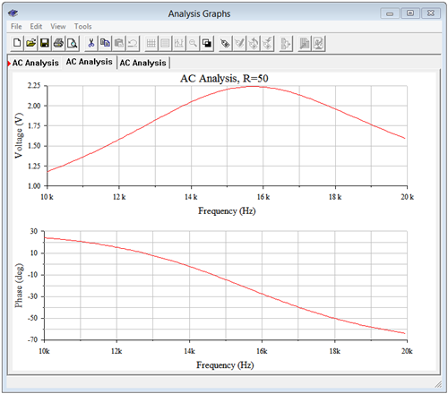
Next, the coil resistance is raised to 50 \(\Omega \), yielding a \(Q\) of only 2. The simulation is run a second time. \(k_p\) drops to 0.866 with this lowered \(Q\) and should produce an \(f_0\) of approximately 13.77 kHz. The plots are shown in Figure \(\PageIndex{18}\), and zoomed in for a better view. From the lower graph it is obvious that the frequency where the curve reaches \(0^{\circ}\) is just below 14 kHz. Accurate measurement yields 13.78 kHz, right in line with the theoretical computation.
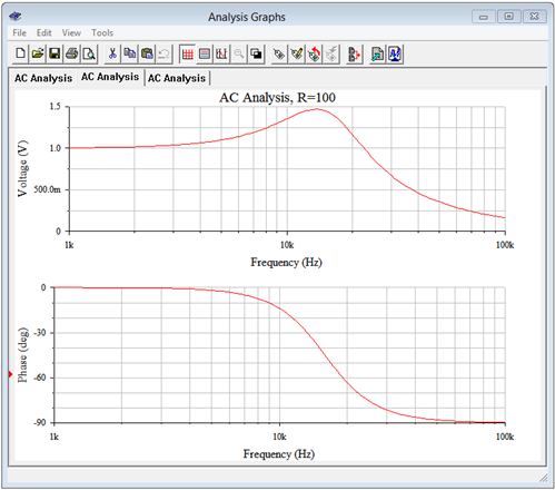
Finally, the coil resistance is increased to 100 \(\Omega \). This drops the circuit \(Q\) to 1 and more importantly, brings \(k_p\) down to 0. The resulting simulation plots are shown in Figure \(\PageIndex{19}\). At first glance the phase plot looks similar to that of Figure \(\PageIndex{17}\), however, notice that the phase scale has changed with \(0^{\circ}\) as the maximum. In fact, the phase shift never quite reaches \(0^{\circ}\). In this regard we can still say that the \(k_p\) equation remains an accurate predictor.
Alternate Definition for Parallel Resonant Frequency
Instead of defining the parallel resonant frequency as the point where the power factor is unity, i.e., where \(X_L\) and \(X_C\) have the same magnitude, it can be defined in terms of the frequency where the magnitude of the impedance is maximum. For high \(Q\) circuits the two definitions produce essentially the same frequency, however, as the circuit \(Q\) decreases into the single digits, the frequency of maximum impedance begins to deviate from both the high \(Q\) idealization and the general unity power factor definition. In fact, the frequency of maximum magnitude is situated between the two. We shall refer to this frequency as \(f_{Z-max}\) to avoid confusion. The formula is2:
\[f_{\text{Z-max}} = f_0 \sqrt{\sqrt{\frac{2}{Q_{circuit}^2} +1} − \frac{1}{Q_{circuit}^2}} \label{8.25} \]
This equation will yield a value between the ideal high \(Q\) case and the unity power factor case. This can be seen in Figure \(\PageIndex{19}\) where there is still an impedance peak (as evidenced by the voltage peak) in spite of the fact that a phase angle of \(0^{\circ}\) is not reached. Furthermore, the frequency of the peak is below that of the high \(Q\) case. Equation \ref{8.25} predicts a peak at 13.6 kHz which agrees with the value obtained from the simulation.
Combination Series and Parallel Resonance
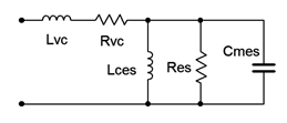
In closing our discussion on resonance we might ask whether or not there are practical, everyday examples of systems exhibiting series and parallel resonance in series-parallel circuits. The answer is yes. A good example is that of a basic dynamic moving coil loudspeaker of the type seen in Chapter 2. This is an electro-mechanical system and thus a proper model has to include the effects of such items as the mechanical losses in the system, the mass of the cone, and the like. One possibility is shown in Figure \(\PageIndex{20}\). \(L_{vc}\) and \(R_{vc}\) are the inductance and resistance of the voice coil. The remaining components model other aspects of the electro-mechanical system. An impedance plot of a typical loudspeaker is shown in Figure \(\PageIndex{21}\).
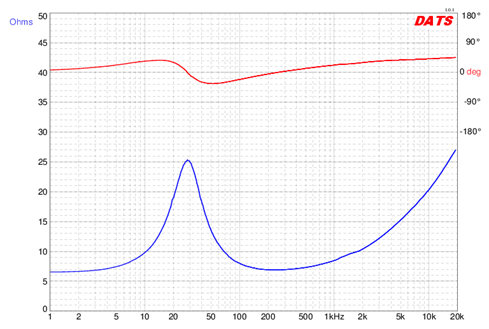
The loudspeaker of Figure \(\PageIndex{21}\) is a medium-size woofer with a nominal impedance of 8 \(\Omega \). First, note the large variation on both the phase and magnitude of the impedance. The parallel items from the model produce an obvious peak in impedance just below 30 Hz. This is referred to as the free air resonance and is denoted by \(f_s\). For this device, the magnitude is over three times the nominal value. Also note that the phase angle is \(0^{\circ}\) at \(f_s\), and that the phase is positive (inductive) below the resonant frequency and negative (capacitive) above it. This behavior is expected from a parallel resonant system. The series elements of the model create the rising impedance that is seen following the dip. Note that the phase angle continues to increase as frequency rises, indicating the growing dominance of the series inductive element.
References
1Note that if this value had been greater than 25 we'd be stuck for a different reason; namely that we'd need to obtain a higher quality inductor because \(Q_{circuit}\) can't be any higher than \(Q_{coil}\).
2For a non-calculus proof, see K. Cartwright, E. Joseph, E. Kaminsky, “Finding the Exact Maximum Impedance Resonant Frequency of a Practical Parallel Resonant Circuit Without Calculus”, Technology Interface International Journal, vol. 11, no. 1, Fall/Winter 2010. [Online Serial]. Available: http://tiij.org/issues/issues/winter...inter_2010.htm [Accessed February 15, 2020 ].