1.2: Paleoclimate

Measurements with modern instruments (the instrumental record) are available only for roughly the past century. This is insufficient to describe the full natural variability of the climate system, which makes attribution of observed changes difficult. We want to know if the changes observed in the recent past are unusual compared to pre-industrial climate variability. If they are it is more likely that they are anthropogenic, if not they could well be natural. Paleoclimate research is also important for a fundamental understanding of how the climate system works. Some paleoclimate changes, e.g. the ice age cycles, were much larger than those during the instrumental record. Thus, we can learn much from paleoclimate data about the impacts of large climate changes.

a) Methods

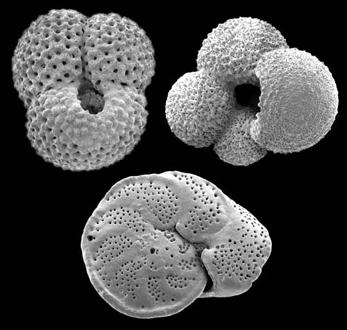
Paleoclimate research is able to extend the instrumental record back in time much further than the instrumental record and has delivered a fascinating history of past climate changes. Most paleoclimate evidence is indirect and based on proxies for climate variables. This evidence is less precise than measurements with modern instruments because of the additional uncertainty in the relation between the proxy and the climate variable. Examples for proxies are pollen (Fig. 1) found in lake sediments that can be used to reconstruct past vegetation cover, which in turn can be related to temperature and precipitation. Similarly, different species of planktic foraminifera prefer different temperatures. Some live in colder waters others prefer warmer waters. Their fossil shells accumulate in sediments, which can be retrieved with a coring device employed from a research vessel. Shells deeper in the sediment are older. If shells of cold-loving foraminfera are found at a site where currently warm-loving species live, it suggests that near surface temperatures in the past have been colder. Mathematical methods have been developed to quantify the temperature changes from the species composition. Other proxies are chemical such as the ratio of magnesium to calcium (Mg/Ca), which is related to temperature, or isotopes of oxygen or carbon in the calcium carbonate shells of foraminifera, which can be used to reconstruct temperature, salinity, ice volume and carbon cycling. Benthic foraminifera live on or in the ocean’s sediments and thus provide useful information on deep ocean properties. Here is an excellent interactive post about paleoclimate proxies.

A

B

Figure \(\PageIndex{1}\): Electron microscope pictures of fossil foraminifera (A, two planktic foraminifera on top and one benthic foraminifera on the bottom) and pollen (B).

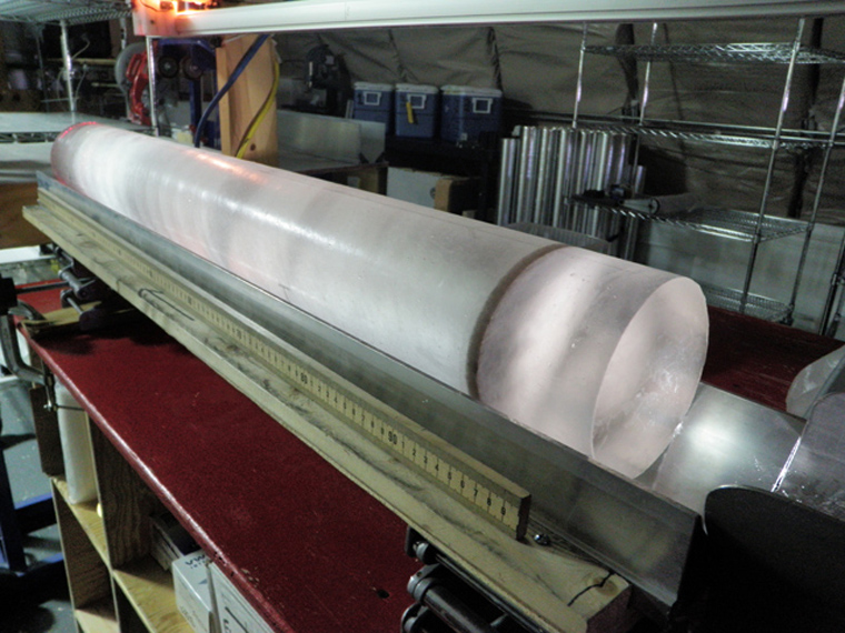
Proxies are found in different archives such as tree-rings, ice-cores, corals, ocean or lake sediment cores that cover different time periods at a range of temporal resolutions (Fig. 2). The  resolution of a record can be quantified as the time difference Δt = t₂ – t₁ between two adjacent samples t₁ and t₂. The smaller Δt the higher the resolution. Written historical accounts can be used to reconstruct past climatic conditions at very high temporal resolution – some ancient documents contain daily weather entries – back to about 1,000 years, but there are only a limited number of such records available. Tree-rings, corals and speleothems (cave deposits such as stalactites and stalagmites) provide reconstructions at annual to decadal resolution (Δt ~ years to decades) back many thousands of years. Ice cores have typically decadal to centennial resolution going back almost a million years for Antarctica and about 100,000 years for Greenland. Ocean sediment cores cover millions of years in the past but usually at low temporal resolution of centennial to millennial timescales (Δt ~ 100s to 1,000s of years).

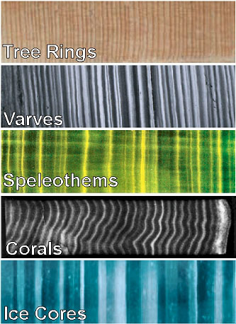
Figure \(\PageIndex{2}\):  Layered paleoclimate archives. Varves are layered sea or lake sediments.

Several methods are used to date samples to construct chronologies of paleoclimate records. Tree-rings are annual layers, which can be counted. Patterns of thin and thick rings can be matched from one tree to another, older one (Fig. \(\PageIndex{3}\)). This way a large number of trees can be used to create a long layer-counted chronology. Layer counting can also be used in other archives with annual layers such as ice cores or lake sediments. Most ocean sediments don’t have annual layers because of bioturbation, which is the mixing of sediments by worms and other organisms that live in the sediment. When organic material is present radiocarbon dating can be used to determine the age of a sample. Radiocarbon (¹⁴C) decays exponentially with a half-life of 5,730 years. Thus, the lower the ratio of radiocarbon to regular carbon (¹⁴C/¹²C) in a sample, the older it is. This ratio can be measured precisely with a mass spectrometer. However, this method can only be used until about 40,000 years before the present because older material has unmeasurably small amounts of ¹⁴C.

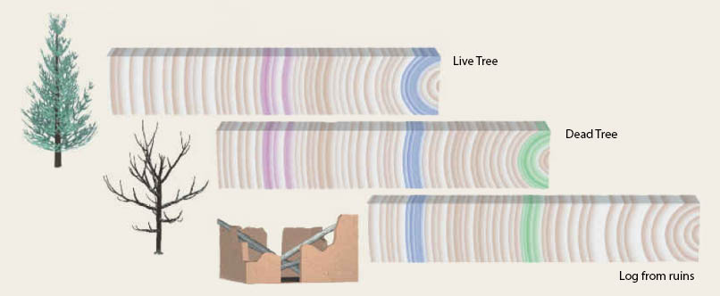
Figure \(\PageIndex{3}\): Long tree ring chronologies can be constructed by matching overlapping patters of different trees.

b) The Last Two Millennia

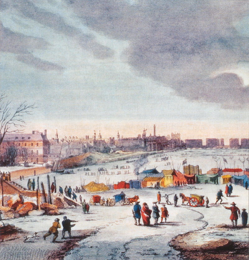
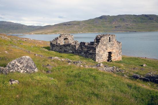
Historical accounts such as pictures of the frozen Thames (Fig. 4) document a period of relatively cold conditions during the 16^th to 19^th centuries in Europe called the Little Ice Age. Conversely, relatively warm conditions during the 9^th to 13^th centuries, called the Medieval Warm Period, may have allowed Vikings to colonize Greenland and travel to North America.

A

B

Figure \(\PageIndex{4}\): A: Picture of the frozen Thames from 1683-84 by Thomas Wyke. B: Ruins of Hvalsey Church from the Greenland settlements of the Norse.

Two recent reconstructions of global temperatures, however, indicate that the Medieval Warm Period was not a global phenomenon (Fig. \(\PageIndex{5}\)). These reconstructions also suggest that there was a long term cooling trend during the past 2,000 years that culminated in the Little Ice Age, which was terminated by a relatively rapid warming during the 20^th century. According to the PAGES 2k reconstruction global average temperature during the three decades from 1971 to 2000 was warmer than at any other 30-year period in the last 1,400 years. This suggests that the recent warming is unusual. The rate of change during the last ~100 years also seems to be unusually fast compared with the previous 2,000 years. The two independent reconstructions agree well in the cooling trend over the past 1,000 years, but the PAGES 2k reconstruction suggests slightly warmer conditions during the first millennium CE (Common Era). The Marcott et al. (2013) dataset is based mostly on lower resolution ocean sediment cores and is therefore smoothed compared to the higher resolution PAGES 2k dataset, which includes mostly land data such as pollen and tree rings.

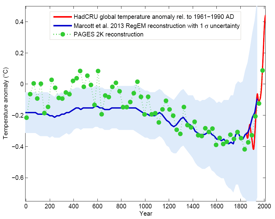
Figure \(\PageIndex{5}\): Global multi-proxy temperature reconstructions from the PAGES 2k project based on 7 continental scale regional reconstructions (green) compared with an independent reconstruction that includes the whole Holocene (Marcott et al., 2013; blue with shaded error range; see also Figure 7) and the instrumental record (red). The PAGES 2k reconstruction represents 30-year averages. It includes many more data than the lower resolution Marcott et al. (2013) reconstruction, particularly for the last 1,000 years. Thus the error range of the PAGES 2k reconstruction is presumably much smaller than that indicated by the blue shading. From RealClimate.

 

c) The Holocene

Fig. \(\PageIndex{6}\) shows the full Holocene (the last 10,000 years) reconstruction of global average temperatures from Marcott et al. (2013). It suggests that the long term cooling trend of the last 2,000 years is part of a longer trend that extends back in time to the middle Holocene around 4,000 BC. The early Holocene from around 8,000 BC to 4,000 BC was relatively warm, similarly to recent decades. (This is debated in the scientific community; a recent paper suggest that it wasn’t warmer during the early Holocene and that biases in proxies related to seasonality are to blame. If this is true, the current warming will be unprecedented for more than 10,000 years, perhaps more than 100,000 years or longer.) The rate of temperature change appears to be much smaller compared with the last 100 years, but the relatively low resolution of the reconstruction leads to smoothing and does not allow a fair comparison with the instrumental record on 100 year timescales.

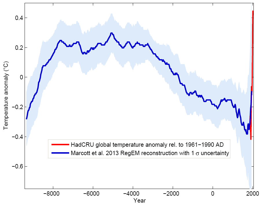
Figure \(\PageIndex{6}\): Holocene global surface temperature reconstruction from Marcott et al. (2013, blue) with shaded error ranges together with the instrumental record (red) as a function of time in years CE. From RealClimate.

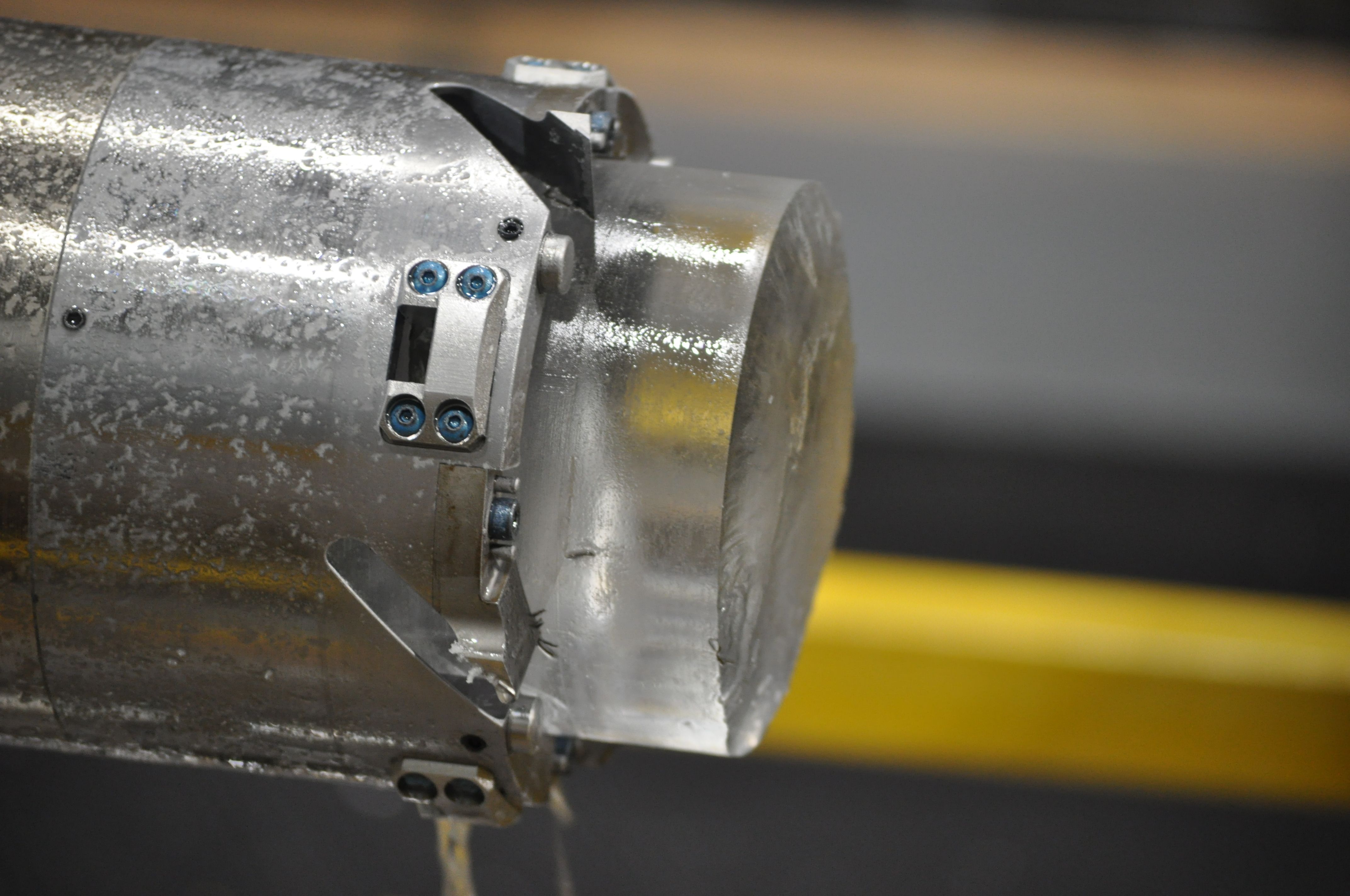
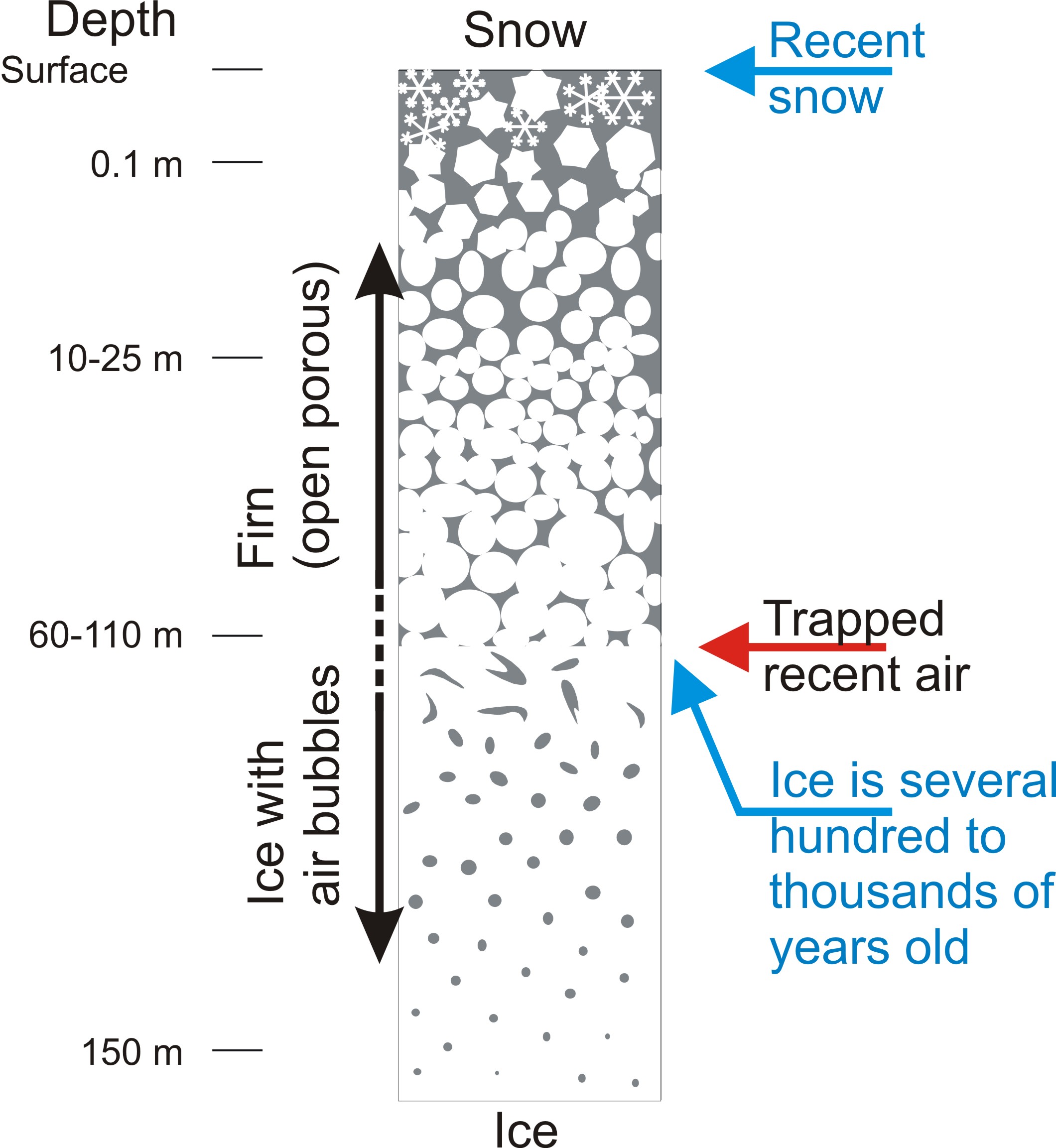
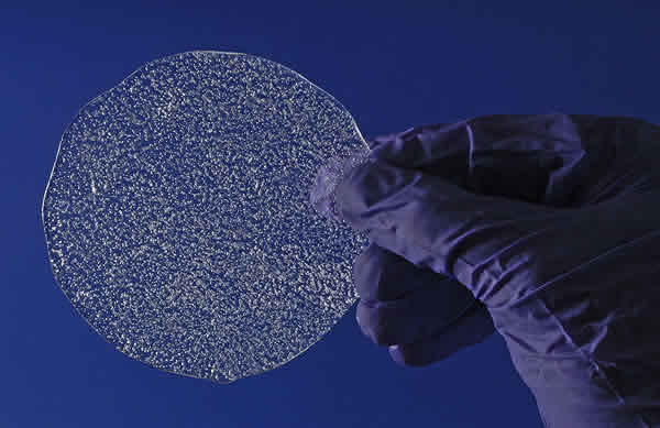
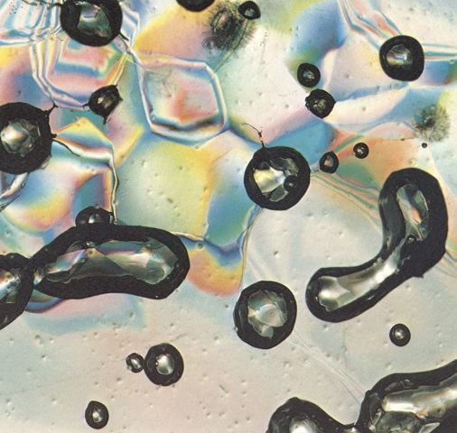
Now let’s have a look at CO₂. Is the observed increase in atmospheric CO₂ during the last 60 years unusual compared to the pre-industrial Holocene? Ice cores can be used to answer this question. When snow accumulates on an ice sheet it compresses to firn and later to ice due to the pressure of the overlaying snow (Fig. 7). During this compaction process small bubbles of air are trapped within the ice. In the lab the air can be extracted from the ice, e.g. by mechanically crushing the ice, and its CO₂ concentration, and other greenhouse gases, can be measured.

 

A

B

C

Figure \(\PageIndex{7}\): Ice cores have been drilled in different locations in Antarctica (top left) using drilling devices like the one depicted here (B). Air gets trapped in the ice through compaction of snow and firn (C). These air bubbles in the ice are visible by eye (D) and in the microscope (E). Sometimes dark ash layers are found in ice cores, which can help to date the ice (F).

D

E

F

Ice cores from Greenland are not suitable for CO₂ reconstructions because they are contaminated by impurities (e.g. dust) that can lead to CO₂ production in the ice. However, Antarctic ice is so pure that it provides excellent records of past atmospheric CO₂ concentrations. Different ice cores have been drilled in Antarctica (Fig. \(\PageIndex{7}\)). The measurements from the youngest ice and firn match up very well with the direct measurements of modern air from Mauna Loa (Fig. 8). Also, the measurements from different ice cores agree with each other (different colored symbols in Fig. \(\PageIndex{8}\)). This indicates that Antarctic ice cores faithfully record past atmospheric CO₂ concentrations. The results show that atmospheric CO₂ concentrations have been relatively constant between about 260 and 280 ppm during the Holocene (the last 10,000 years). It was only during the last 200 years that CO₂ concentrations started to increase. Thus, we have answered the question posed above and conclude that the CO₂ increase during the last 200 years is very unusual and has not happened before during the last 10,000 years. We also know that burning of fossil fuels has increased dramatically after the industrial revolution (1760-1840). In the carbon cycle chapter below, more evidence will be presented that demonstrates that the subsequently observed CO₂ increase was indeed due to human activities such as the burning of fossil fuels.

 

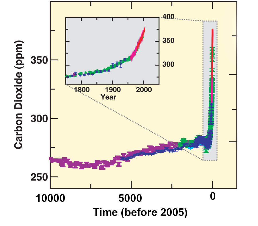
Figure \(\PageIndex{8}\): Ice core CO₂ measurements of ancient air. The different colors indicate different ice cores. The inset zooms into the last 200 years and includes in red the modern air measurements from Mauna Loa (see Figure 8 in Chapter 2). Note that the ice core measurements agree well with the modern data where they overlap. From IPCC (2007).

Other greenhouse gases have also been measured in air extracted from ice cores. Methane (CH₄) and nitrous oxide (N₂O) show a very similar behavior to CO₂, such that their concentrations were relatively constant throughout the Holocene around 700 ppb and 260 ppb, respectively, and increased dramatically during the last 200 years to values around 1,700 and 310 ppb, respectively (IPCC, 2007).

 

d) The Ice Ages

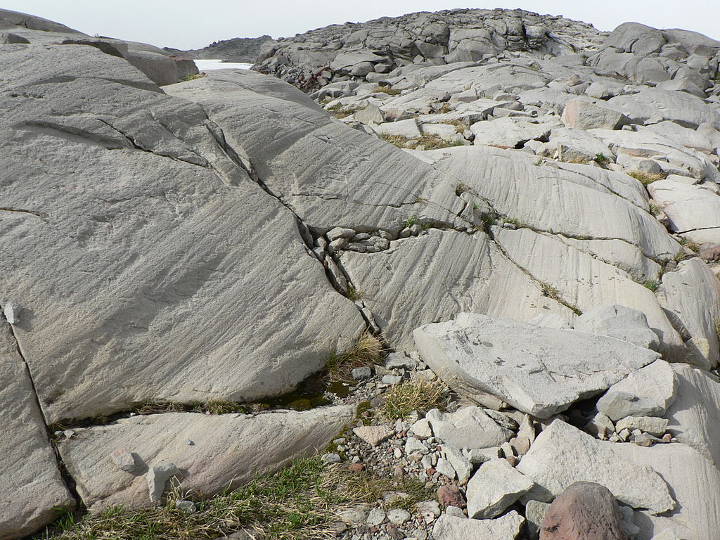
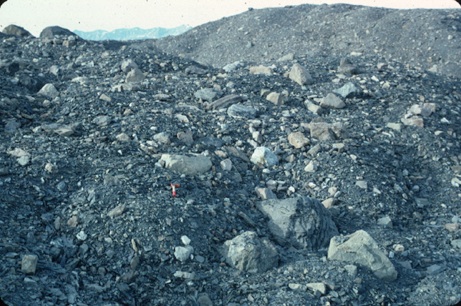
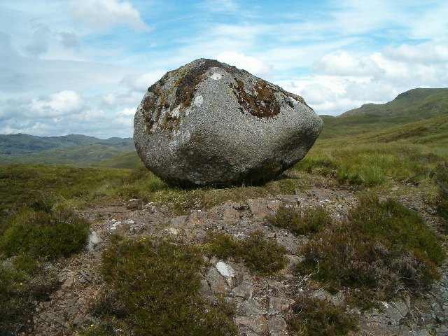
Fig. \(\PageIndex{6}\) already hints at a cold period before the Holocene. Indeed we now know that for a long time Earth had been in an ice age, or glacial state, before the current warm period of the Holocene begun. But it was only in the 19^th century that scientists realized that Earth has experienced ice ages on a global scale. This discovery was made by Louis Agassiz, a Swiss geologist, who hypothesized that not only Alpine glaciers were advanced but also large ice sheets moved south from northern Europe and America leaving glacial landforms behind (Fig. \(\PageIndex{9}\)). For a fascinating and more detailed account of this discovery the reader is referred to Imbrie and Imbrie (1979).

 

A

B

Figure \(\PageIndex{9}\): Glacial Landforms. Top: Polished bedrock with striations indicate a glacier was moving over it. The glacier incorporates rocks into its base and by pushing them over the underlying bedrock creates grooves. This example is from Mount Rainier National Park. A: Moraines (this example is from Svalbard) are glacial deposits formed at the side (lateral moraines) or end (terminal moraines) of a moving glacier. B: Erratic boulders like this one from Scotland, many miles from a possible bedrock source, have been attributed by Louis Agassiz to the action of ice-age glaciers.

During the height of the last ice age, the Last Glacial Maximum (LGM) roughly 20,000 years ago, large additional ice sheets covered parts of North America and northern Europe (Fig. 10). The Laurentide Ice Sheet was more than 3 km thick and covered all of what is now Canada and part of the northern United States reaching as far south as New York City, Chicago, and Seattle. The Eurasian (or Fennoscandian) Ice Sheet covered all of Scandinavia, much of the British isles, the Baltic Sea, and surrounding land areas from northeastern Germany to northwestern Russia. Mountain glaciers also descended further down valleys and often into the low lands.

Figure 10: Reconstructions of ice sheets (contour lines show 500 m elevation differences) and surface temperature differences from modern (color scale in K) for the Last Glacial Maximum. From PAGES news.

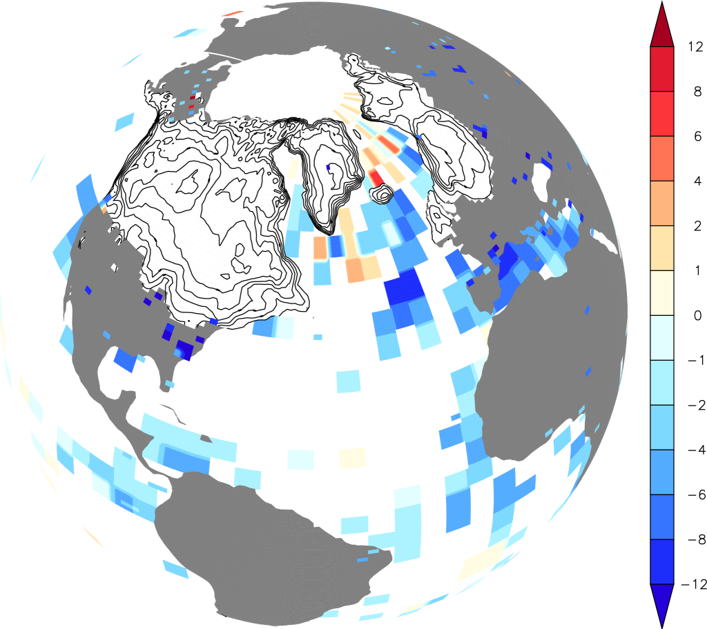
Figure \(\PageIndex{10}\): Reconstructions of ice sheets (contour lines show 500 m elevation differences) and surface temperature differences from modern (color scale in K) for the Last Glacial Maximum. From PAGES news.

Because so much more water was locked up as ice on land, sea level was 120 m lower during the LGM than it is today. Imagine your favorite beach of today. There was no water there at the LGM. Explore with NOAA’s interactive bathymetry viewer how much further it would have been to the water during the LGM at your favorite beach.

The LGM is a well-studied time period in paleoclimate research, and we have a wealth of data available. Ice cores show lower concentrations of atmospheric greenhouse gases such as CO₂ (180 ppm vs 280 ppm during the late pre-anthropogenic Holocene; Fig. \(\PageIndex{10}\)) and methane. Vegetation reconstructions show that forests were replaced by tundra and grasslands over large parts of the mid- to high latitudes (Prentice et al., 2011). We also know from ice and ocean sediment cores that the air was dustier. Temperature proxies show colder temperatures almost everywhere (Fig. \(\PageIndex{10}\)). However, temperature changes were not the same everywhere. Temperature changes over large parts of the tropical and subtropical oceans were rather small. Globally-averaged sea surface temperatures have been estimated to be only 2°C cooler than the present (MARGO, 2009). Land areas in the tropics experienced moderate cooling of about 3°C (Bartlein et al., 2011). The largest cooling of more than 8°C occurred over land at mid-to-high latitudes and over Antarctica (Fig. \(\PageIndex{11}\)). Globally averaged surface air temperature has been estimated to be 4°C colder during the LGM (Annan and Hargreaves, 2013). More recent, yet unpublished studies suggest 5°C indicating some uncertainty in these estimates. These authors also suggest that on average the cooling over land was 3 times larger than over the oceans. The land-sea contrast and polar amplification =are similar to what we’ve seen in observed warming over the past century (Fig. 2 in Chapter 2). This suggests that those are robust properties of the climate system.

Box 1: Oxygen Isotopes

Isotopes are variations of the same element with a different number of neutrons, which leads to a different mass (Fig. B\(\PageIndex{1}\)). Since different isotopes of the same element have the same number of electrons (yellow circles in Fig. B\(\PageIndex{1}\)) they react chemically identically or very similar.

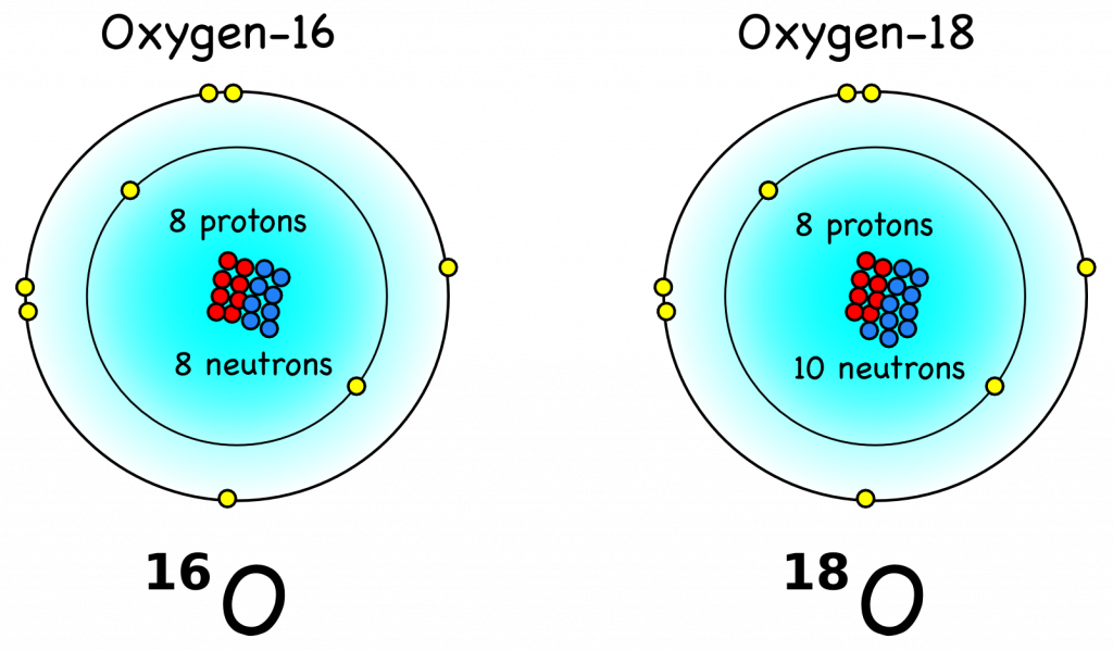
Figure B\(\PageIndex{1}\): Oxygen’s most common (99.8%) isotope oxygen-16 (\( ^{16}O \)) has 8 protons (red) and 8 neutrons (blue) such that its mass is 16 atomic units. Oxygen-18 (\( ^{18}O \)) has two additional neutrons, which makes it (18 – 16)/16 = 12.5% heavier than \( ^{16}O \). It is also much rarer (0.2%) than \( ^{16}O \). From Montessori Muddle.

Water molecules (H₂O) with \( ^{18}O \)  are (20 – 18)/18 = 11% heavier than those with \( ^{18}O \). The mass of a molecule affects how likely it will participate in a phase change such as evaporation or condensation. Water molecules at a certain temperature in the water phase have a distribution of kinetic energy \(\frac{1}{2}mv^{2}\). Some are a little faster, others are a little slower. Only the fastest will be able to leave the water phase and make it to the vapor phase (air). (Here is a nice youtube video explaining this in a little bit more detail.) Because the mass of a heavy water molecule is larger, its velocity, on average, must be smaller in order to have the same kinetic energy. Therefore, the heavier isotopes will remain in the liquid phase more often than the lighter isotopes. This process is called fractionation. It leads to an accumulation of heavy water isotopes in the ocean and relatively more light water isotopes in the air.

Here is an analogy. Imagine a number of black and white soccer balls are lined up at the center line of a soccer field. The black balls are slightly heavier than the white balls. Now a player will shoot the balls, one after another, alternatively black and white, towards the goal. When he/she is done you count the balls that made it across the goal line. Will there be more black or white balls? Yes, indeed, more white balls, because they are lighter and they fly farther due to larger velocities put in by the player who exerts about the same amount of energy for each shot. In this analogy the white balls are the light isotopes.

Isotopes are usually expressed as delta values such as \( \delta ^{18}O = \left ( R-R_{std} \right )/R_{std} \), where \( R= ^{18}O/^{16}O \)is the heavy over light ratio of a sample, relative to that of a standard \( R_{std} \).   Fig. B2 illustrates how fractionation during evaporation and condensation affects the isotope values of water, vapor, and ice in the global hydrological cycle.

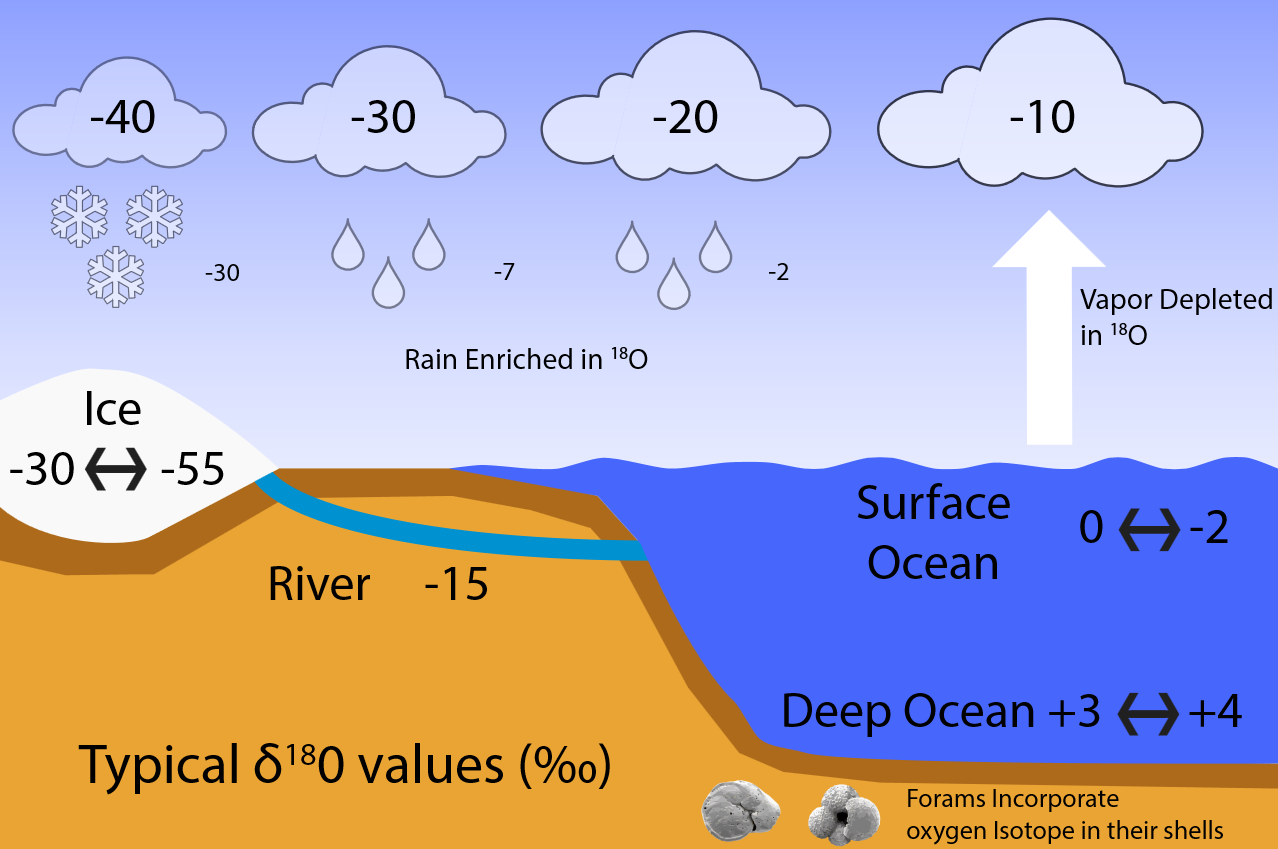
Figure \(\PageIndex{1}\): Typical δ\( ^{18}O \) values (in permil). Surface ocean water has δ\( ^{18}O \) values of around zero. Due to fractionation during evaporation less heavy isotopes make it into the air, which leads to negative delta values of around -10 ‰. Condensation prefers the heavy isotopes for reasons analogous to evaporation. In this example the first precipitation thus has a δ18O value of about -2 ‰, the remaining water vapor will be further depleted in \( ^{18}O \) relative to \( ^{16}O \) thus that its δ\( ^{18}O \) value is approximately -20 ‰. Any subsequent precipitation event further depletes \( ^{18}O \). This process is known as Rayleigh distillation and leads to very low δ\( ^{18}O \) values of less than -30 ‰ for snow falling onto ice sheets. Thus, ice has very negative δ\( ^{18}O \) of between -30 and -55 ‰. Deep ocean values today are about +3 to +4 ‰. During the LGM, as more water was locked up in ice sheets, the remaining ocean water became heavier in δ\( ^{18}O \) by about 2 ‰. We know this because foraminifera build their calcium carbonate (CaCO3) shells using the surrounding sea water. Thus they incorporate the oxygen isotopic composition of the water into their shells which are preserved in the sediments and can be measured in the lab.

 

We conclude that paleoclimate data from the LGM show that Earth was dramatically different from today, with large ice sheets, low sea level, and different vegetation. These changes happened even though the global average temperatures changed only by 4-5°C. This is comparable to changes projected for some future scenarios.

Geologic evidence such as that shown in Fig. \(\PageIndex{9}\)is abundant only for the last major glaciation because each glacial advance erases evidence from previous glaciations. However, because of our friends, the foraminifera, we know many details of previous glaciations. How can that be? Foraminifera live in the ocean. Well, as explained in the box, the δ¹⁸O of sea water records the amount of ice volume and thus sea level. Since foraminifera record the δ¹⁸O of sea water in their shells, we can amazingly reconstruct past ice volume from tiny shells found in mud on the ocean floor.

Fig. \(\PageIndex{11}\) shows that there were about 9 glacial-interglacial cycles during the past 800,000 years. Most of the time sea level was lower than today, during some of the glacial maxima by more than 120 m. Ice core records show that glacial periods were always associated with low atmospheric CO₂ concentrations and low temperatures in Antarctica. CO₂ concentrations varied between about 180 ppm during glacial maxima and 280 ppm during interglacials. The correlation between these completely independent datasets, one from Antarctic ice cores, the other from deep sea foraminifera, is astounding. It demonstrates that climate and the carbon cycle are tightly interlinked. High CO₂ concentrations are always associated with warm temperatures, high sea level, and low ice volume. This indicates the importance of atmospheric CO₂ concentrations for climate but it also suggests that climate impacts the carbon cycle and causes changes in CO₂.

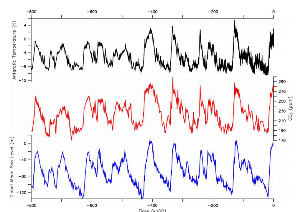
Figure \(\PageIndex{11}\): Glacial-interglacial Cycles. Top: Antarctic temperature anomaly estimated from deuterium ratios measured in the ice (Jouzel et al., 2007). Deuterium (D) is the heavy hydrogen isotope ²H. In H₂O it works similar to the heavy oxygen isotope as a local temperature proxy. Center: Atmospheric CO₂ concentrations from ice cores (Lüthi et al., 2008). Bottom: Global sea level changes (ΔSL = [δ¹⁸O – 3.2 ‰]×[-120 m / 1.69 ‰]) estimated from oxygen isotopes (δ¹⁸O) measured in benthic foraminifera from deep-sea sediments (Lisiecki and Raymo, 2004). This is a key figure.

Closer inspection of leads and lags shows that during the last deglaciation CO₂ and Antarctic temperature lead global temperature, which suggests that CO₂ is an important forcing mechanism for the warming (Shakun et al., 2012). But we also know that climate affects the carbon cycle. For example, CO₂ is more soluble in colder water, which causes the ice age ocean to take up additional carbon from the atmosphere. Another likely reason for the lower glacial CO₂ concentrations in the atmosphere is iron fertilization. The colder glacial atmosphere was also dustier. Dust contains iron and thus iron delivery to currently iron limited regions such as the Southern Ocean was increased during the ice age. This intensified phytoplankton growth and the biological pump, which describes processes of sinking and sequestering of carbon in the deep ocean. Our recent research indicates that about half (~45 ppm) of the glacial-interglacial CO₂ variations can be explained by temperature and another 25-35 ppm by iron fertilization (Khatiwala et al., 2019). However, this topic is not settled and subject to ongoing research. More about how climate can affect CO₂ will be discussed in the carbon cycle chapter. For now let’s just conclude that climate and the carbon cycle are tightly linked.

But what causes glacial-interglacial cycles? They are caused by changes in Earth’s orbit around the sun, which affects the seasonal distribution of incoming solar radiation. This theory was first proposed in 1938 by Serbian astronomer Milutin Milankovich, who calculated variations in Earth’s orbital parameters and linked those to past ice ages. Earth’s orbit can be described by three parameters (Fig. \(\PageIndex{12}\)). The eccentricity E is the deviation from a perfectly circular orbit. Earth’s orbit is a slight ellipse although it is close to circular. E varies on ~100,000 year cycles between zero and 0.06. The tilt T, or obliquity, describes the angle between Earth’s axis of rotation and the ecliptic, which is the plane of Earth’s orbit around the sun. It is currently T = 23.5° but it varies between 24.5° and 22.5° on a 40,000 year cycle. Precession P is the wobble of Earth’s axis, like the wobble of a top. Currently we’re closest to the sun in January, which corresponds to the axis tilted towards the left in Fig. \(\PageIndex{12}\). P varies on a 23,000 year cycle and is strongly modulated by eccentricity. These variations are caused by gravitational forces from the other planets, particularly Jupiter and Saturn.

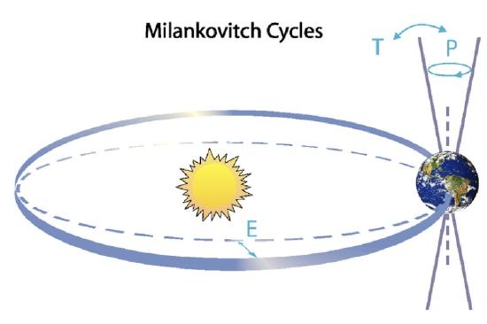
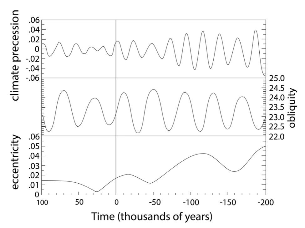
Figure \(\PageIndex{12}\): Milankovitch Cycles. Top: Earth’s orbit around the sun is determined by eccentricity (E), tilt (T) or obliquity, and precession (P). Bottom: Variation of Earth’s orbital parameters through time. Negative numbers towards the left show the past and positive numbers show the future.

Milankovich’s theory is that summer insolation in the northern hemisphere controls the waxing and waning of the ice sheets. When summer insolation is high, all snow from the previous winter will melt away. When summer insolation is low, some snow survives and during the next winter more snow accumulates. In this way, an ice sheet can grow. The northern hemisphere is important because that is where the major land masses are, where additional ice sheets can grow. The Antarctic ice sheet did not fundamentally change during the ice ages, although it grew somewhat bigger during the ice ages and shrunk a bit during interglacials and the Patagonian ice sheet was much smaller than those in the north.

The Milankovich theory was essentially confirmed by spectral analysis of deep sea δ¹⁸O data, which shows all the predicted periodicities (Hays et al., 1976). However, exactly when and why ice ages start and end remain active topics of research.

While the Milankovich theory explains the cyclicity and timing of glacial-interglacial cycles it does not explain their amplitudes (how much global average temperatures have changed). Simulations with gobal climate models show that the amplitude of glacial-interglacial temperature changes can only be reproduced if CO₂ changes are accounted for (e.g. Shakun et al., 2012). This leads us to conclude that CO₂ changes are an important (feedback) factor in determining glacial-interglacial temperature changes although the ultimate cause of the ice age cycles are Earth’s orbital cycles.

Questions

• What are paleoclimate proxies?
• What is a paleoclimate archive?
• Which paleoclimate record has higher resolution: record A, which has data every 100 years, or record B, which as data every 1,000 years?
• What is a chronology?
• Name two methods that are used to date paleoclimate samples?
• How much colder was global average surface air temperatures during the LGM?
• How much colder was global average sea surface temperatures during the LGM?
• How much lower was global sea level during the LGM?
• How much lower was atmospheric CO₂ during the LGM compared to the pre-industrial late Holocene?
• What is the Milankovich theory?
• How do we know the extent of glaciation during the last ice age?
• How do we know sea level and ice volume during previous glaciations?

Videos

Lecture: Last 2,000 Years, Holocene

Lecture: Ice Ages & Isotopes

Lecture: Milankovitch

 

 

References

Annan, J. D., and J. C. Hargreaves (2013), A new global reconstruction of temperature changes at the Last Glacial Maximum, Clim Past, 9 (1), 367-376, doi:10.5194/cp-9-367-2013.

Bartlein, P., et al. (2011), Pollen-based continental climate reconstructions at 6 and 21 ka: a global synthesis, Clim Dynam, 37, 775-802, doi:10.1007/s00382-010-0904-1.

Hays, J. D., J. Imbrie, and N. J. Shackleton (1976), Variations in Earths Orbit – Pacemaker of Ice Ages, Science, 194 (4270), 1121-1132, doi:10.1126/science.194.4270.1121.

IPCC (2007) Summary for Policymakers. In: Climate Change 2007: The Physical Science Basis. Contribution of Working Group I to the Fourth Assessment Report of the Intergovernmental Panel on Climate Change [S. Solomon, D. Qin, M. Manning, Z. Chen, M. Marquis, K. B. Averyt, M. Tignor, H. L. Miller, (eds.)]. Cambridge University Press, Cambridge, United Kingdom, New York, NY, USA.

Imbrie, J., and K. P. Imbrie (1979) Ice ages: solving the mystery, Harvard University Press, Cambridge Massachusetts and London, England, 224 pp, ISBN 9780674440753.

Jouzel, J., et al. (2007) Orbital and millennial Antarctic climate variability over the past 800,000 years, Science, 317 (5839), 793-796, doi:10.1126/science.1141038.

Khatiwala, S., A. Schmittner and J. Muglia (2019) Air-sea disequilibrium enhances ocean carbon storage during glacial periods Science Advances, 5(6), doi: 10.1126/sciadv.aaw4981.

Lisiecki, L. E., and M. E. Raymo (2005), A Pliocene-Pleistocene stack of 57 globally distributed benthic δ¹⁸O records, Paleoceanography, 20(1), PA1003, doi:10.1029/2004pa001071.

Lüthi, D., et al. (2008), High-resolution carbon dioxide concentration record 650,000-800,000 years before present, Nature, 453(7193), 379-382, doi:10.1038/nature06949.

Marcott, S. A., J. D. Shakun, P. U. Clark, and A. C. Mix (2013), A reconstruction of regional and global temperature for the past 11,300 years, Science, 339(6124), 1198-1201, doi:10.1126/science.1228026.

MARGO, et al. (2009), Constraints on the magnitude and patterns of ocean cooling at the Last Glacial Maximum, Nat Geosci, 2(2), 127-132, doi:doi:10.1038/Ngeo411.

PAGES 2k Consortium, M. Ahmed, K. J. Anchukaitis, A. Asrat, H. P. Borgaonkar, M. Braida, B. M. Buckley, U. Büntgen, B. M. Chase, D. A. Christie, E. R. Cook, M. A. J. Curran, H. F. Diaz, J. Esper, Z.-X. Fan, N. P. Gaire, Q. Ge, J. Gergis, J. F. González-Rouco, H. Goosse, S. W. Grab, N. Graham, R. Graham, M. Grosjean, S. T. Hanhijärvi, D. S. Kaufman, T. Kiefer, K. Kimura, A. A. Korhola, P. J. Krusic, A. Lara, A.-M. Lézine, F. C. Ljungqvist, A. M. Lorrey, J. Luterbacher, V. Masson-Delmotte, D. McCarroll, J. R. McConnell, N. P. McKay, M. S. Morales, A. D. Moy, R. Mulvaney, I. A. Mundo, T. Nakatsuka, D. J. Nash, R. Neukom, S. E. Nicholson, H. Oerter, J. G. Palmer, S. J. Phipps, M. R. Prieto, A. Rivera, M. Sano, M. Severi, T. M. Shanahan, X. Shao, F. Shi, M. Sigl, J. E. Smerdon, O. N. Solomina, E. J. Steig, B. Stenni, M. Thamban, V. Trouet, C. S. M. Turney, M. Umer, T. van Ommen, D. Verschuren, A. E. Viau, R. Villalba, B. M. Vinther, L. von Gunten, S. Wagner, E. R. Wahl, H. Wanner, J. P. Werner, J. W. C. White, K. Yasue, E. Zorita (2013) Continental-scale temperature variability during the past two millennia, Nat Geosci. 6, 339-346, doi:10.1038/ngeo1797.

Prentice, I. C., S. P. Harrison, and P. J. Bartlein (2011), Global vegetation and terrestrial carbon cycle changes after the last ice age, New Phytol, 189(4), 988-998, doi:10.1111/j.1469-8137.2010.03620.x.

Shakun, J. D., P. U. Clark, F. He, S. A. Marcott, A. C. Mix, Z. Y. Liu, B. Otto-Bliesner, A. Schmittner, and E. Bard (2012), Global warming preceded by increasing carbon dioxide concentrations during the last deglaciation, Nature, 484(7392), 49-54, doi:10.1038/Nature10915.