11.3: The Case Study1

This application study has to do with validating the design of a new manufacturing cell particularly with respect to staffing requirements as well as work in process inventory levels and throughput. An initial value for the number of workers required as well as an initial assignment of workers to workstations can be determined by standard, straightforward cellular manufacturing computations.

A simulation study is required to validate that the number of workers and their assignment to workstations determined by the cellular manufacturing analysis will allow the cell to meet its throughput requirements. The effect on throughput as well as WIP due to other assignments and numbers of workers can be evaluated.

Factors not included in the initial calculations can be taken into account in the simulation model. Task and walking times as well as the time between arrivals of parts may be random variables. Cell operating rules for co-ordination between the activities of multiple workers as well as part arrivals to the cell is necessary.

11.3.1 Define the Issues and Solution Objective

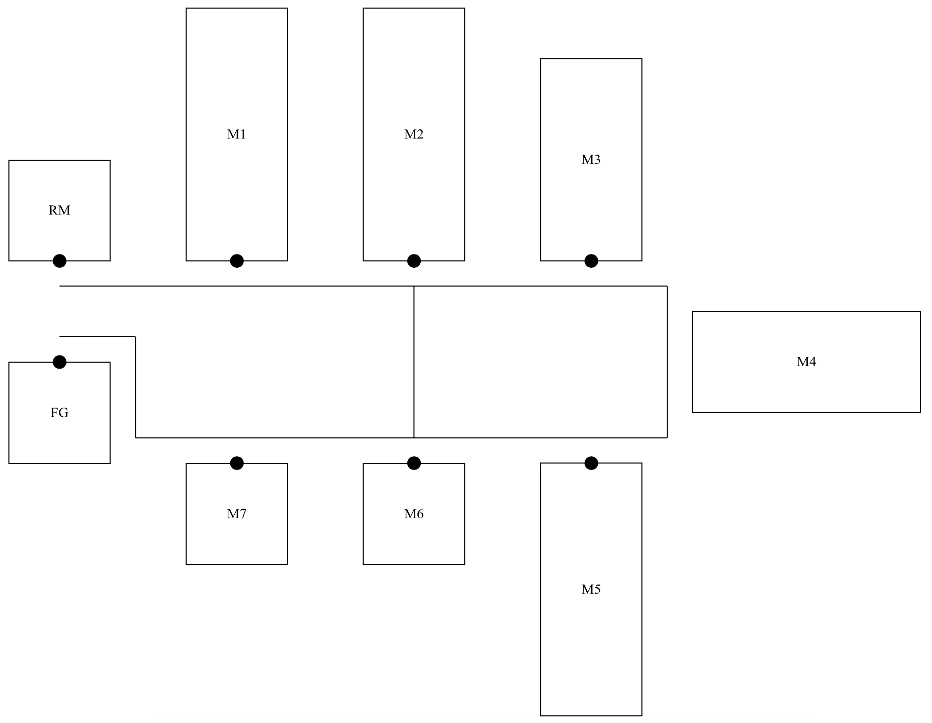
A new manufacturing cell is being implemented. The design of the cell is shown in Figure 11-3. The cell consists of seven workstations each with one machine as well as a raw material inventory of parts to process. A completed finished goods inventory is included.

The work area at each work station is shown by a heavy dot. The worker walking path in the cell is shown by a line. Note that a worker may walk directly between workstation M2 and workstation M6. The worker who is responsible for a machine also walks the part from the immediately preceding workstation or inventory. The worker responsible for workstation M7 also walks a completed part to the finished goods inventory.

Table 11-1 provides basic data concerning the operation at each workstation. All times are in seconds. Manual times represent the constant standard times.

---

¹ Professor Jon Marvel defined this application problem as well as providing other invaluable assistance. Mr. Joel Oostdyk implemented a prototype model. Ms. Michelle Vette provided some excellent insight for improving the application problem.

---

Table 11-1: Workstation Processing Information (Times in Seconds)
Workstation / Task Name	Workstation / Task ID	Initiation Time (Manual)	Operation Time (Automated)	Removal Time (Manual)	Total Time
Pick Up Raw Material	RM	4			4
Turn Outer Diameter	M1	4	23	3	30
Bore Inner Diameter	M2	5	41	4	50
Face Ends	M3	4	32	4	40
Grind Outer Diameter	M4	3	29	3	35
Grind Outer Diameter	M5	3	29	3	35
Inspect	M6	14			14
Drill	M7	3	24	3	30
Place in Finished Goods Inv.	FG	5			5
Total		45	168	20	233

Figure 11-3: Manufacturing Cell

The cell is responsible for producing 1000 units of one part each day. The cell will operate for two shifts of 460 minutes each. Thus the takt time is computed using equation 11-1 to be:

\(\ takt time =\frac{\text { available work time per day}}{\text { demand per day }}=\frac{460\ X\ 2}{1000}=0.920 \quad minutes = 55.2 seconds\)

The number of workers needed in the cell can be determined as follows. Notice that the total manual operation time, the time a worker is required, is shown in Table 11-1 to be 65 ( = 45 + 20) seconds. This total time divided by the takt time (65 / 55.2) is between 1 and 2. Thus, a minimum of two workers is required.

In addition, worker walking time must be taken into account. It is highly desirable to have workers walk a circular route. Walking time plus manual task time for the route must be less than the takt time. Any assignment should seek to balance the manual operation plus walking time among the workers. Workers walk on the average of 2 feet per second.

Table 11-2 shows the walking distance between adjacent workstations.

Table 11-2: Walking Distances Between Workstations
Workstation / Task ID	Workstation / Task ID	Walking Distance (feet)
RM	M1	7
M1	M2	7
M2	M3	7
M2	M6	8
M3	M4	8
M4	M5	8
M5	M6	7
M6	M7	7
M7	FG	10

One possible assignment using two workers is the following (Assignment A):

Worker 1: RM, M1, M2, M7, FG
(Task time, 31 seconds; walking time, 21.5 seconds; total time, 52.5 seconds)

Worker 2: M3, M4, M5, M6
(Task time, 34 seconds; walking time, 19 seconds; total time, 53 seconds)

The standard work cell design procedures did not take into account the following factors that may proof to be significant in the operation of the cell:

1. Walking times are modeled as triangularly distributed random variables with the minimum equal to 75% of the mean and the maximum equal to 125% of the mean. Based on the VUT equation, this could add to the cycle time and WIP in the cell. Thus, the effect of random walking times needs to assessed.
2. There is concern as to whether a constant time between arrivals of parts from another area of the plant can be achieved. The practical worst case assumptions (Hopp and Spearman, 2007) lead to modeling the time between arrivals as exponentially distributed with mean equal to the takt time. Again by the VUT equation, considering the time between arrivals to be a random variable could add to the cycle time and WIP in the cell. Thus, the performance of the cell for the case of a constant interarrival time for parts must be compared to the case of an exponentially distributed interarrival time.
3. The following operational rule will be employed. Worker 1 will wait at the raw material station and worker two will wait at station M2 until a part is available to walk to the next station.

The simulation study must show that the above assignment is feasible, given the three operational factors. Furthermore, the utilization of workers in the proposed assignment scheme is very high, 95% for worker 1 and 96% for worker 2. It is possible that it is not feasible to effectively co-ordinate the tasks of both workers and the operations of the machines. Thus as alternative assignment was proposed (Assignment B).

Worker 1: RM, M1, M2 (Total time, 41 seconds)

Worker 2: M3, M4, M5 (Total time, 43 seconds)

Worker 3: M6, M7, FG (Total time, 42 seconds)

Each worker has several tasks. Each task must be performed in sequence as the worker walks around the cell. For example, worker 1 in assignment A has the following sequence of tasks:

1. Wait for part at RM
2. Process part at RM
3. Move part from RM to M1
4. Unload previous part from M1
5. Initiate part on M1
6. Move unloaded part from M1 to M2
7. Remove part from M2
8. Initiate part unloaded from M1 on M2
9. Walk without a part to M6
10. Wait for an inspected part
11. Walk with an inspected part from M6 to M7
12. Remove part from M7
13. Initiate inspected part on M7
14. Walk with part removed from M7 to FG
15. Process part at FG
16. Walk with no part to RM

The following priorities are of fundamental importance in achieving one piece flow and not loosing machine capacity. These are reflected in the worker task sequence.

1. After removing a part from a machine, a worker will start another part on the same machine if one is available before performing any other task.
2. After walking a part from a preceding workstation or inventory and upon arriving at the next workstation, the worker will initiate the operation on a part, if the machine is available.

From the point of view of a part, the work cell will operate in the following way. Parts arrive to the raw material inventory from another area of the plant. The average time between arrivals is equal to the takt time.

Parts move through the same processing steps at each workstation except M6: initiation on the machine by a worker, automated processing by the machine, and removal from the machine by a worker. Processing at M6 is consists of one manual inspection step.

Workers move parts between machines as well as from the raw materials inventory to the first workstation and from the last workstation to the finished good inventory. Part processing and movement is constrained by the availability of workers and machines.

11.3.2 Build Models

The model will be built from the perspective of worker movement. A worker walks between stations in a prescribed route and performs one or two tasks at each station. Parts reside in inventories. A typical station has the following inventories: waiting for initiation on a machine, waiting for unloading from a machine, and waiting to be walked to the next station. A worker action changes the number of parts in one of the inventories.

The model consists of four processes:

1. Arrival of parts to the raw material inventory.
2. Worker 1
3. Worker 2
4. Automated processing on a machine which does not require worker assistance.

The following inventories exist in the model.

1. Workstations M1 - M5 and M7: waiting for initiation on a machine (WaitInitialize), waiting for unloading from a machine (WaitUnload), and waiting to be walked to the next station (WaitWalk).
2. Workstation M6: waiting to be walked to the next station (WaitWalk).
3. Raw materials: (RMInv)
4. Finished goods: (FGInv)

Entities in the arrival of parts process and the automated processing process represent parts. For the latter process, entity attributes are:

1. ID: ID number of the workstation station where automated processing occurs: 1, 2, 3, 4, 5, or 7.
2. OpTime: Processing time at the workstation.

The worker is the only entity in the worker process. This entity has one attribute:

1. WithPart: 1, if the worker has a part when walking between workstations and zero otherwise.

The following variables are used in the model.

1. WIPCell: The total number of parts in the work cell
2. WalkTime (9, 9): Average walking time between each pair of stations, FG (8), and RM(9).

The part arrival process follows. A part arrives and the RM inventory is increased by 1 as well as the total WIP in the cell.

---

Define Arrivals: \(\ \quad \quad\)Parts \(\ \quad \quad\quad \quad\)Time of first arrival: \(\ \quad \quad\quad \quad\)Time between arrivals: \(\ \quad \quad\quad \quad\)Number of arrivals:	0 Exponentially distributed with a mean of 55.2 seconds Infinite
Define Resources: \(\ \quad \quad\)M(7)/1 with states (Busy, Idle)	// Workstation resources
Define Entity Attributes: \(\ \quad \quad\)WorkstationID \(\ \quad \quad\)OperationTime \(\ \quad \quad\)WithPart	// ID number (1, ..., 7) of workstation to process a part // Time to process a part at a workstation // The number of parts carried by a worker from station to station (0, 1)
Define State Variables \(\ \quad \quad\)WIPCell \(\ \quad \quad\)RMInv \(\ \quad \quad\)FGInv \(\ \quad \quad\)WaitInitialze(7) \(\ \quad \quad\)WaitUnload(7) \(\ \quad \quad\)WaitWalk(7) \(\ \quad \quad\)WalkTime (9, 9)	// The amount of work-in-process in the cell // Raw material inventory // Finished goods inventory // Number of items waiting for initialization at a workstation // Number of items waiting unloading at a workstation // Number of items waiting to be walked to the next workstation // Inter-station walk times
Process PartArrival Begin \(\ \quad \quad\)WIPCell ++ \(\ \quad \quad\)RMInv ++ End

---

The automated processing process is exactly the same as the single worker station process discussed previously. Upon the completion of processing, the number of parts waiting to unload is increased by one.

---

Process AutomatedMachine
Begin
\(\ \quad \quad\)WaitUntil M(WorkstationID)/1 is Idle in Queue QM(WorkstationID)
\(\ \quad \quad\)Make M(WorkstationID)/1 Busy
\(\ \quad \quad\)Wait for OperationTime
\(\ \quad \quad\)Make M(WorkstationID)/1 Idle
\(\ \quad \quad\)WaitUnload(WorkstationID) ++
End

---

The process for Worker 1 starting at RM through arrival at workstation M2 follows. Note that the worker waits at RM for a part to carry to workstation M1. Otherwise, the worker will carry a part between workstations, unload a part or initialization a part only if a part is available. Each inventory is updated as the worker acts.

---

Process Worker1 Begin // From raw material inventory to M1 Wait until RMInv > 0 Wait for 4 seconds RMInv - WithPart = 1 Wait for triangular WalkTime(9,1)*75%, WalkTime(9,1), WalkTime(9,1)*125% WaitInitialize (1) ++ // Processing at M1 If WaitUnload(1) > 0 then Begin // Unload Part at M1 Wait until M(1)/1 is Idle in Queue QM(1) Make M(1)/1 Busy Wait for 3 seconds Make M(1)/1 Idle WaitUnload(1)-- WaitWalk(1)++ End If WaitInitialize(1) > 0 then Begin // Initialize Part at M1 Wait until M(1)/1 is Idle in Queue QM(1) Make M(1)/1 Busy Wait for 4 seconds Make M(1)/1 Idle WaitInitialize(1)-- // Process part in parallel with worker walking ID = 1 OperationTime = 23 Clone to AutomatedMachine End If WaitWalk(1) > 0 then Begin // Walk with part WaitWalk(1) - WithPart = 1 End Else WaitPart = 0 Wait for triangular WalkTime(1,2)*75%, WalkTime(1,2), WalkTime(1,2)*125% WaitInitialize(2) ++ End

// Wait for the next part // Processing at raw material inventory // Update raw material inventory // Worker carrying one part // To M1 // Add to initialize inventory at M1 // No part // To M2 // Arrive at M2 and Update Inventory

---

11.3.3 Identify Root Causes and Assess Initial Alternatives

Experimentation with the model is used to address the issues previously raised with respect to performance of the cell.

1. The effect of random walking times.
2. The effect of random times between arrivals.
3. The number of workers used in the cell: 2 or 3.
4. The effect of operational rules for workers.

The amount of work in process in the cell should be very low. Thus, the total WIP in the cell will be used as a performance measure. The WIP at RM is also of interest. In addition, a trace showing the time sequence of worker movements and activities is desired for both model and cell design validation.

The design of the simulation experiment is shown in Table 11-3. Since the cell is assigned a certain volume of work each day, a terminating experiment of duration one work day (920 minutes) is used. Twenty replicates are used. Random number streams are needed for worker walking time as well as the time between arrivals.

Table 11-3: Simulation Experiment Design for the Manufacturing Cell

Element of the Experiment	Values for This Experiment
Type of Experiment	Terminating
Model Parameters and Their Values	1. Time between arrivals (random or constant) 2. Number of workers (2 or 3)
Performance Measures	1. WIP in the cell 2. WIPatRM
Random Number Streams	1. Worker walking time 2. Time between arrivals
Initial Conditions	One part at each station
Number of Replicates	20
Simulation End Time	920 minutes (one day)

Initial conditions of that reflect the principle of one piece flow are appropriate. Thus, there is one part at each station initially. At all stations except M6, the part is placed in the WaitUnload inventory. At station M6, the part is placed in the WaitWalk inventory.

Simulation results for the cases when 2 workers are used are shown in Table 11-4.

The cell performs very well when the time between arrivals is constant. The maximum number of parts in the cell is 9, one more than the number of stations plus the raw material inventory. At most 1 part is in the raw material inventory. However, when the time between arrivals is exponentially distributed, large maximum WIP sizes are seen both in the cell in general and in the raw material inventory. Note, however, that the difference between the maximum WIP in the cell and the maximum WIP in the raw material inventory for each replicate is either 7 or 8. Thus, WIP is properly restricted to the raw material inventory.

Table 11-4: Work in Process in the Cell and in RM – Two Workers Cases

	Maximum WIP in Cell			Maximum WIP in RM
Replicate	Constant Time between Arrivals	Random Time between Arrivals	Difference	Constant Time between Arrivals	Random Time between Arrivals	Difference
1	9	52	43	1	44	43
2	9	65	56	1	58	57
3	9	89	80	1	81	80
4	9	51	42	1	43	42
5	9	30	21	1	22	21
6	9	37	28	1	29	28
7	9	75	66	1	67	66
8	9	39	30	1	31	30
9	9	31	22	1	23	22
10	9	47	38	1	39	38
11	9	51	42	1	44	43
12	9	62	53	1	54	53
13	9	72	63	1	64	63
14	9	48	39	1	40	39
15	9	22	13	1	14	13
16	9	37	28	1	29	28
17	9	31	22	1	23	22
18	9	25	16	1	17	16
19	9	79	70	1	71	70
20	9	31	22	1	23	22
Average	9	48.7	39.7	1	40.8	39.8
Std. Dev.	0	19.4	19.4	0	19.5	19.5
99% CI Lower Bound	9	36.3	27.3	1	28.3	27.3
99% CI Upper Bound	9	61.1	52.1	1	53.3	52.3

Table 11-5 contains a portion of the trace for worker 1 for one replicate of the constant time between arrivals case. The trace shows the actions the worker takes from processing a part at RM to processing the next part at RM. The time between starting the processing of a part at RM and return was 52.06 seconds, only slightly less than the expected time of 55.2 seconds. Thus, there is some evidence that the worker can perform all assigned tasks in less than the takt time. The trace shows that worker performs all assigned tasks in the required sequence. Thus, model and system design validation evidence is obtained.

Table 11-5: Worker 1 Action Trace

Simulation Time	Worker	Workstation	Action
55.20	Worker1	RM	Start
59.20	Worker1	RM	End
62.64	Worker1	M1	Arrive
62.64	Worker1	M1	Unload Start
65.64	Worker1	M1	Unload End
65.64	Worker1	M1	Initialize Start
69.64	Worker1	M1	Initialize End
73.46	Worker1	M2	Arrive
73.46	Worker1	M2	Unload Start
77.46	Worker1	M2	Unload End
77.46	Worker1	M2	Initialize Start
82.46	Worker1	M2	Initialize End
85.98	Worker1	M6	Arrive
89.86	Worker1	M7	Arrive
89.86	Worker1	M7	Unload Start
92.86	Worker1	M7	Unload End
92.86	Worker1	M7	Initialize Start
97.86	Worker1	M7	Initialize End
103.13	Worker1	FG	Arrive
108.13	Worker1	FG	End
110.26	Worker1	RM	Arrive
110.40	Worker1	RM	Start

The same results for the case where three workers are used are shown in Table 11-6 along with a comparison to the two workers case. For the random time between arrivals case, the average maximum WIP in the cell is 32.0 when three workers are used. This is notably less than the average when two workers are used: 48.7. Similarly, the average maximum WIP at RM is less when three workers are used: 22.0 versus 40.8. The reductions in WIP in the cell and at station RM due to using three workers instead of two are statistically significant at an approximate 99% confidence level. The approximate 99% confidence intervals of the difference do not contain zero.

Table 11-6: Work in Process in the Cell and in RM – Three Workers Case with Comparison to the Two Workers Case for Random Times Between Arrivals

	Maximum WIP in Cell			Maximum WIP at RM
Replicate	Two Workers	Three Workers	Difference	Two Workers	Three Workers	Difference
1	52	37	15	44	27	17
2	65	32	33	58	22	36
3	89	49	40	81	39	42
4	51	31	20	43	21	22
5	30	24	6	22	14	8
6	37	35	2	29	25	4
7	75	48	27	67	38	29
8	39	28	11	31	18	13
9	31	24	7	23	14	9
10	47	25	22	39	15	24
11	51	28	23	44	18	26
12	62	37	25	54	27	27
13	72	38	34	64	28	36
14	48	32	16	40	22	18
15	22	22	0	14	12	2
16	37	31	6	29	21	8
17	31	26	5	23	16	7
18	25	25	0	17	15	2
19	79	39	40	71	29	42
20	31	28	3	23	18	5
Average	48.7	32.0	16.8	40.8	22.0	18.9
Std. Dev.	19.4	7.6	13.3	19.5	7.6	13.4
99% CI Lower Bound	36.3	27.1	8.2	28.3	17.1	10.3
99% CI Upper Bound	61.1	36.8	25.3	53.3	26.8	27.4

11.3.4 Review and Extend Previous Work

Management was pleased with the results of the simulation experiments. The cell appears to work as designed using standard cellular manufacturing calculations when the time between arrivals is constant.

Exponentially distributed times between arrivals result in large maximum WIP levels. Controls placed on cell operations, in particular requiring a worker to wait at RM for a part, resulted in the all of the excess WIP residing in the RM. Thus, the cell appears to be capable of operating effectively even in the presence of random variation in part arrival.

11.3.5 Implement the Selected Solution and Evaluate

It was decided to implement the cell with two workers. If the high utilization of the two workers constrained the actual operation of the cell, a third worker could be added.