1.2: First-Order ODE Models

Electrical, mechanical, thermal, and fluid systems that contain a single energy storage element are described by first-order ODE models.

Let \(u(t)\) denote a generic input, \(y(t)\) denote a generic output, and \(\tau\) denote the time constant; then, a generic first-order ODE model is expressed as: \[\tau \frac{dy(t)}{dt} +y(t)=u(t) \nonumber \]

The time constant, \(\tau\), denotes the time when the system response to a constant input rises to 63.2% of its final value. The time constant is measured in \(\left[sec\right]\).

Examples

Example \(\PageIndex{1}\)

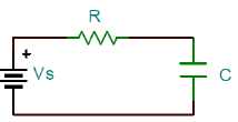
A series RC network is connected across a constant voltage source, \(V_\rm s\) (Figure 1.2.1). Kirchhoff’s voltage law (KVL) is used to model the circuit behavior as: \(v_{R} +v_{C} =V_s\)

In the above capital letters represent constant values and small letters represent time-varying quantities.

Let \(v_{C} =v_{0}\) define the circuit output; then, \(v_{R} =iR=RC\frac{dv_{0} }{dt}\), hence

\[RC\frac{dv_{0} (t)}{dt} +v_{0} (t)=V_s \nonumber \]

The time constant of the RC circuit is given as: \(\tau = RC\).

Figure \(\PageIndex{1}\): A series RC circuit driven by a constant voltage source.

Example \(\PageIndex{2}\)

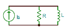
A parallel RL network is connected across a constant current source, \(I_\rm s\) (Figure 1.2.2). The circuit is modeled by a first-order ODE, where the variable of interest is the inductor current, \(i_{L}\), and Kirchhoff’s current law (KCL) is applied at a node to obtain: \(i_{R} +i_{L} =I_\rm s\).

By substituting \(i_{R} =\frac{v}{R} =\frac{L}{R} \frac{di_{L} }{\rm dt}\) we obtain the ODE description of the RL circuit as:

\[\frac{L}{R} \frac{di_{L} (t)}{dt} +i_{L} (t)=I_s \nonumber \]

The time constant of the RL circuit is given as: \(\tau = \frac{L}{R}\).

Figure \(\PageIndex{2}\): A parallel RL circuit driven by a constant current source.

Example \(\PageIndex{3}\)

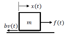
The motion of an inertial mass, \(m\), acted by a force, \(f(t)\), in the presence of kinetic friction, represented by \(b\), is governed by Newton’s second law of motion (Figure 1.2.3). Let \(v\left(t\right)\) represent the velocity; then, the resultant force on the mass element is: \(f-bv\). Hence

\[m\frac{dv(t)}{dt} +bv(t)=f(t) \nonumber \]

The time constant for the mechanical model is: \(\tau =\frac{m}{b}\), which describes the rate at which the velocity builds up in response to a constant force input.

Figure \(\PageIndex{3}\): Motion of an inertial mass with applied force under surface friction.

Example \(\PageIndex{4}\)

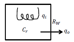
A model for room heating is developed as follows (Figure 1.2.4): let \(q_{i}\), denote heat inflow, \(C_{r}\) denote the thermal capacity of the room, \(\theta _{r}\) denote the room temperature, \(\theta _{a}\) denote the ambient temperature, and \(R_{w}\) denote a thermal resistance representing wall insulation; then, the heat energy balance equation is given as:

\[C_{r} \frac{d\theta_{r} }{dt} +\frac{\theta_{r} -\theta_{a} }{R_{w} } =q_{i} \nonumber \]

In terms of the temperature differential, \(\Delta \theta =\theta _{r} -\theta _{a}\), the governing ODE is:

\[R_{w} C_{r} \frac{ d\Delta \theta }{ dt} +\Delta \theta =R_{w} q_{i} \nonumber \]

By comparing with the generic first-order ODE model, \(\tau \frac{\rm dy}{\rm dt} +y=u\), the thermal time constant is described as: \(\tau =R_{w} C_{r}\). Further, the temperature is measures in \([{}^\circ C]\), heat flow is measured in \([W]\), thermal capacitance is measured in \(\left[\frac{J}{{}^\circ C}\right]\), and thermal resistance is measured in \(\left[\frac{{}^\circ C}{W}\right]\).

Figure \(\PageIndex{4}\): A model of room heating with heat source and outflow through the walls.

Example \(\PageIndex{5}\)

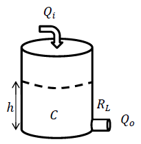
A cylindrical reservoir is filled with an incompressible fluid supplied from an inlet with a controlled exit through a hydraulic valve at the bottom (Figure 1.2.5).

Let \(P\) denote the hydraulic pressure, \(A\) denote the area of the reservoir, \(h\) denote the height, \(V\) denote the volume, \(\rho\) denote the mass density, \(R_{l}\) denote the valve resistance to the fluid flow, \(q_{ in} ,\; q_{out}\) denote the volumetric flow rates, and \(g\) denote the gravitational constant; then, the base pressure in the reservoir is obtained as: \[P=P_{atm} +\rho gh=P_{atm} +\frac{\rho g}{A} V \nonumber \]

The reservoir capacitance is defined as: \(C_{h} =\frac{dV}{dP} =\frac{A}{\rho g}\); then, the governing equation for hydraulic flow through the reservoir is given as: \[C_{h} \frac{dP}{dt} =q_{ in} -\frac{P-P_{atm} }{R_{l} } \nonumber \]

In terms of the pressure difference, the equation is written as: \[R_{l} C_{h} \frac{d\Delta P}{ dt} +\Delta P=R_{l} q_{in} . \nonumber \] By comparing with generic first-order ODE model, \(\tau \frac{dy}{dt} +y=u\), the hydraulic time constant is described as: \(\tau =R_{w} C_{r}\).

Further, by substituting: \(\mathit{\Delta}P=\rho gh\) and \(C_h=\frac{A}{\rho g}\), we can equivalently express the ODE in terms of the liquid height, \(h\left(t\right)\), in the reservoir as:

\[AR_l\frac{dh}{dt}+\rho gh=R_lq_{in} \nonumber \]

In the above, the hydraulic pressure is measures in \(\left[\frac{N}{m^2}\right]\), volumetric flow is measured in \(\left[\frac{m^3}{s}\right]\), hydraulic capacitance is measured in \(\left[\frac{m^5}{N}\right]\), and flow resistance is measured in \(\left[\frac{Ns}{m^5}\right]\).

Figure \(\PageIndex{5}\): A hydraulic reservoir with flow in and flow out through bottom valve.

Solving First-Order ODE Model 

Consider the response of a first-order ODE model: \(\tau \frac{dy\left(t\right)}{dt}+y\left(t\right)=u(t)\) to a step forcing function.

By applying the Laplace transform with initial conditions: \(y\left(0\right)=y_0\), we obtain an algebraic equation:

\[\tau \left(sy\left(s\right)-y_0\right)+y(s)=u(s) \nonumber \]

We assume a unit step input \(u\left(t\right)\), where \(u\left(s\right)=\frac{1}{s}\); then, the output is solved as:

\[y\left(s\right)=\frac{1}{s\left(\tau s+1\right)}+\frac{\tau y_0}{\tau s+1} \nonumber \]

We use partial fraction expansion (PFE) to express the output as:

\[y\left(s\right)=\frac{1}{s}-\frac{\tau }{\tau s+1}+\frac{\tau y_0}{\tau s+1} \nonumber \]

By using inverse Laplace transform, we obtain the time-domain solution to the ODE as:

\[y\left(t\right)=1+\left(y_0-1\right)e^{-t/\tau },\ \ t\ge 0 \nonumber \]

Let the steady-state value of the output be denoted as: \(y_{\infty }={\mathop{lim}_{t\to \infty } y(t)\ }\); then, the step response of a general first-order ODE model is expressed as:

\[y\left(t\right)=\left[y_{\infty }+\left(y_0-y_{\infty }\right)e^{-t/\tau }\right]u\left(t\right) \nonumber \]

In the above, \(u\left(t\right)\) denotes a unit step function, used to show causality, i.e., the response is valid for \(t\ge 0\).

Transfer Function

The transfer function description of a dynamic system is obtained from the ODE model by the application of Laplace transform assuming zero initial conditions. The transfer function describes the input-output relationship in the form of a rational function, i.e., a ratio of two polynomials in the Laplace variable \(s\).

A first-order ODE model with input \(u(t)\) and output \(y(t)\) is described as: \(\tau \frac{\rm dy(t)}{\rm dt} +y(t)=u(t)\).

For the first-order model, application of Laplace transform with zero initial conditions gives: \((\tau s+1)y(s)=u(s)\).

The resulting input–output transfer function is given as:

\[\frac{y(s)}{u(s)} =\frac{1}{\tau s+1} \nonumber \]

Output Response

For zero initial conditions, \(y_0=0\), the output is expressed as:

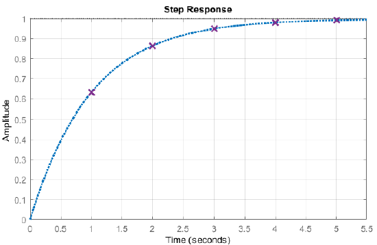
\[y\left(t\right)=\left(1-e^{-t/\tau }\right)u\left(t\right) \nonumber \]

The system response for \(\tau =1\,sec\) is plotted in Figure 1.5.

The output values at selected times, \(t=k\tau ,\ \ k=0,1,\dots\) are compiled in the following table. By convention, the output is assumed to have reached steady-state when it attains 98% of its final value. Hence, the settling time of the system is expressed as: \(t_s=4\tau\).

Table 1.1: The step response of a first-order model at selected time instances.

Time	Output value
0	\(y\left(0\right)=0\)
1\(\tau\)	\(1-e^{-1}\cong 0.632\)
2\(\tau\)	\(1-e^{-2}\cong 0.865\)
3\(\tau\)	\(1-e^{-3}\cong 0.950\)
4\(\tau\)	\(1-e^{-4}\cong 0.982\)
5\(\tau\)	\(1-e^{-5}\cong 0.993\)

Figure \(\PageIndex{6}\): Response of a first-order ODE model (\(\tau=1 sec\)).

pkg load control
s=tf('s');
Gs=1/(s+1);
step(Gs), hold
plot(1:5,1-exp(-(1:5)),'x')