
6.2: Measures of Performance
- Page ID
- 24414

In the frequency response design methods, the measures of performance include relative stability, described in terms of gain and phase margins, error constants, sensitivity and complementary sensitivity functions, etc. These are described below.
It is assumed that the loop transfer function \(KGH(j\omega )\) is minimum-phase, i.e., its poles and zeros are located in the closed left half-plane (CLHP) including the \(j\omega\)-axis.
Relative Stability
In frequency domain design, the relative stability of the feedback loop is described in terms of the gain and the phase margins.
The gain margin (GM) is the maximum amount of loop gain that can be added to the feedback loop (by the controller) without compromising stability.
On the Bode magnitude plot, the GM is indicated as: \(GM=-{\left|KGH\left(j{\omega }_{pc}\right)\right|}_{dB}\), where \(\omega _{\rm pc}\)is the phase crossover frequency, i.e., the frequency at which \(\phi (\omega _{\rm pc} )=-180^{\circ }\).
In the MATLAB Control Systems Toolbox, the ‘margin’ command is used to obtain the GM and PM as well as the gain and phase crossover frequencies on the Bode plot. The command is invoked after defining the loop transfer function using 'tf' or 'zpk' command.
On the Nyquist plot, \({\omega }_{pc}\) is marked by the negative real-axis crossing of \(KGH\left(j\omega \right)\), i.e., let \(G\left({\omega }_{pc}\right)=g\angle -180{}^\circ\); then, \(GM=g^{-1}\).
The phase margin (PM) is the maximum amount of phase that can be added to the feedback loop (by the controller) without compromising stability.
On the Bode phase plot, the PM is indicated as: \(\rm PM=180^{\circ } +\phi (\omega _{\rm gc} )\), where \(\omega _{\rm gc}\) is the gain crossover frequency, i.e., the frequency defined by \(|G(j\omega _{\rm gc} )|=1\).
On the Nyquist plot, the PM is indicated when the plot enters the unit circle, i.e., assume that \(KGH\left(j\omega \right)=1\angle -\phi\), then the phase margin is given as: \({\rm PM}=180^{\circ } -\phi\).
A loop transfer function with pole excess (\(n-m\ge 3\)) has a finite gain margin, i.e., \(0<{\rm GM}<\infty\). The loop transfer function with (\(n-m=2\)) may have a finite GM.
The return difference is described by one minus the loop gain. At the input to the plant, the return difference is 1+KGH(j\omega). The minimum value of the return difference is \(\min_\omega |1+KGH(j\omega )|\).
For minimum-phase plants, the closed-loop stability depends on the Nyquist plot keeping a finite distance from the \(-1+j0\) point. The closest distance of \(KGH(j\omega)\) from the \(-1+j0\) point indicates the minimum return difference with respect to \(G(s)\). The minimum return difference is a measure of the robustness of the control loop to parameter variations in \(G(s)\).
Examples
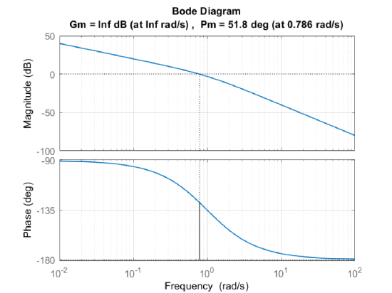
Let \(K\)\(G(s)=\frac{1}{s(s+1)}\); then, from the bode plot, we have \({\rm GM}=\infty\) and \({\rm PM}=51.8^{\circ }\).
From Fig. 6.1.1, the minimum return difference is \(\min_{\omega}|1+KG(j\omega)|=1\).
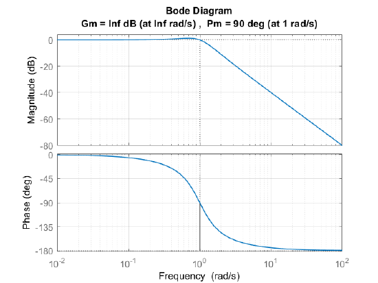
Let \(K\)\(G(s)=\frac{1}{s^2+s+1}\); then, we have \({\rm GM}=\infty\, dB\) and \({\rm PM}=90^{\circ }\).
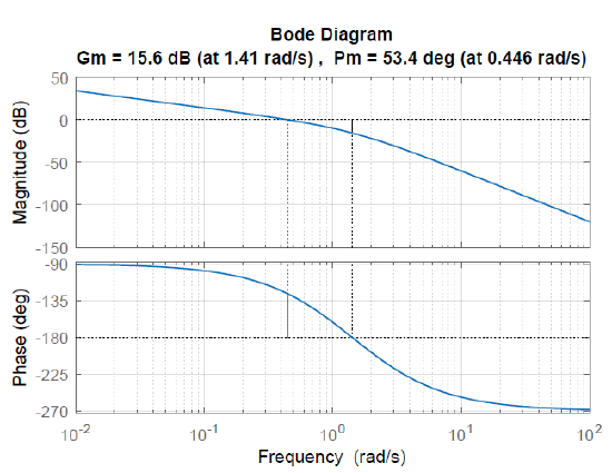
Let \(K\)\(G(s)=\frac{2}{s(s+1)(s+2)}\); then, we have \({\rm GM}=15.6\, dB\) and \({\rm PM}=53.4^{\circ }\).
Closed-Loop System Response
Damping ratio. The damping ratio of the dominant poles in the closed-loop transfer function is related to the phase margin.
In particular, for a prototype second-order transfer function: \(KGH(j\omega )=\frac{\omega _{n}^{2} }{j\omega \, \left(j\omega +2\zeta \omega _{n} \right)}\), the gain crossover occurs at: \(\omega _{gc} =k\omega _{n}\), where \(k=\sqrt{\sqrt{4\zeta ^{4} +1} -2\zeta ^{2} }\), whereas \(\phi _{m} =\tan ^{-1} \left(\frac{2\zeta }{k} \right)\).
In the range of \(0.5<\zeta <0.9\), the approximate relation is given as: \({\phi }_m\cong {{tan}^{-1} \left(\frac{6\zeta }{3.3-2\zeta }\right)\ },\;\;0.5<\zeta <0.9\). As an example, in order to have a \(\zeta =0.7\), we may design the system for a \(PM\cong 65.6^{\circ }\).
Settling time. The settling time of the closed-loop system step response is related to the phase margin. For a second order transfer function, the settling time \(t_s\) and the phase margin \(\phi _\rm m\) are related as: \(\tan \phi _m =\frac{2\zeta \omega _{n} }{\omega _{\rm gc} } =\frac{8}{t_\rm s \omega _{\rm gc} }\).
Bandwidth. The closed-loop bandwidth is bounded as: \(\omega _{n} \le \omega _{B} \le 2\omega _{n} .\)
In particular, for systems with low damping, \(\omega _{B} \cong \omega _{n} .\)
The bandwidth is related to the rise time \(t_{r}\) of the closed-loop system step response as: \(\omega _{\rm B} t_{r} \approx 1\) or \(t_{r} \cong 1/\omega _{\rm B}\).
In particular, in the case of second-order systems (\(0.6<\zeta <0.9\)), the rise time can be approximated as: \(t_{r} \cong \frac{3\zeta }{w_{n} } .\)
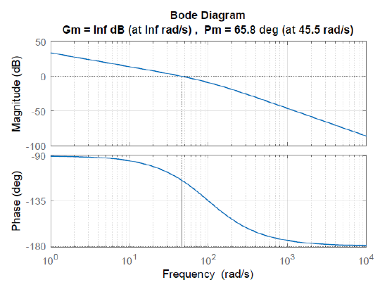
We consider the model of a small DC motor, given as: \(G(s)=\frac{500}{s^{2} +110s+1025} .\)
Assume that a PI compensator for the model is defined as: \(K(s)=\frac{K(s+10)}{s}\). Then, for \(K=10\), we have closed-loop roots located at: \(s=--50\pm j50.4\).
The Bode plot of the loop gain with compensator in the loop displays a phase margin of \(\phi _\rm m =65.8^{\circ }\), which corresponds to a closed-loop damping ratio of \(\zeta =0.7\).
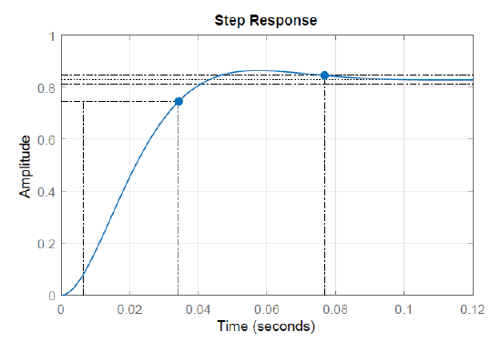
The step response of the compensated system displays a rise time of \(t_{r} =0.028s\) and a settling time of \(t_{s} =0.077s\). The predicted value of the settling time is: \(t_\rm s =\frac{8}{\omega _{gc} \tan \phi _\rm m } =0.078s.\)
Error Constants and System Type
The position and velocity error constants for a unity-gain feedback control system are defined as:
\[K_{\rm p} ={\mathop{\lim }\limits_{s\to 0}} KG(s)\; ,\; \; \; K_{\rm v} ={\mathop{\lim }\limits_{s\to 0}} sKG(s).\; \nonumber \]
These constants can be inferred from the Bode plot at follows: The position error constant is given by the low frequency asymptote on the Bode magnitude plot, that is, \(K_{p} ={\mathop{\lim }\limits_{s\to 0}} \left|KG(j\omega )\right|\).
The velocity error constant is given as the slope of the low frequency asymptote on the Bode magnitude plot, that is, \(\; \; {\mathop{\lim }\limits_{s\to 0}} \left|KG(j\omega )\right|\; =\frac{\; K_{v} }{\omega } .\)
The system type is inferred by the slope of the Bode magnitude plot in the low frequency region. Thus, a slope of \(0dB\) implies a type \(0\) system; a slope of \(-1\), i.e., \(-20\ dB\)/decade implies a type \(1\) system, etc.
System Sensitivity
The sensitivity of the closed-loop transfer function, \(T(j\omega )\), to variations in the plant transfer function, \(G(j\omega )\), is given as:
\[S_{G}^{T} (j\omega )=\frac{\partial T/T}{\partial G/G} =\frac{1}{1+KGH(j\omega )} \nonumber \]
Keeping the sensitivity small over a frequency band requires a high loop gain, \(KGH(j\omega )\). In general, increasing the loop gain decreases the stability margins, i.e., a trade-off exists between the sensitivity and relative stability requirements.
In the context of robust control, the closed-loop transfer function \(T\left(j\omega \right)\) is referred as complementary sensitivity function.
The sensitivity and the complementary sensitivity are fundamentally constrained as: \(S(j\omega )+T(j\omega )=1\).The control system designers generally aim for high loop gain at low frequencies to obtain \(T(j\omega )\cong 1\). The loop gain is reduced at high frequencies to raise the stability margins.
Loopshaping is a graphical technique that aims to impart a desired loop shape to the plot of \(KGH(j\omega )\) by adding compensator poles and zeros to the loop.