
9.3: Tracking PI Controller Design
- Page ID
- 24431

Tracking PI Controller Design
The tracking system design by using a feedforward gain to cancel the tracking error is not robust to changes in plant parameters. A robust tracking system design requires addition of an integrator to the feedback loop (Figure 9.3.1).
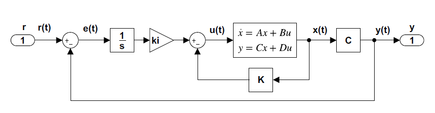
A proportional-integral (PI) type control law using state feedback is defined as: \[u(t)=-{\bf k}^{T} {\bf x}(t)+k_{i} \int (r-y)\rm dt \nonumber \] where \(k_\rm i\) represents the integral gain. The integrator operates on the error signal: \(e=r-y\). The integral controller forces the error signal to zero in the steady-state.
Let \(x_a (t)\) denote the integrator output; then, the integrator state equation is given as: \[\dot{x}_a =r-y=r-{\bf c}^{T} {\bf x} \nonumber \]
An augmented system model is formed by adding the integrator output to the set of state variables; the resulting model with \(n+1\) variables is described as:
\[\left[\begin{array}{c} {\dot{\bf x}} \\ {\dot{x}_a } \end{array}\right]=\left[\begin{array}{cc} {\bf A} & {0} \\ {-{\bf c}^T } & {0} \end{array}\right]\left[\begin{array}{c} {x} \\ {x_a } \end{array}\right]+\left[\begin{array}{c} {\bf b} \\ {0} \end{array}\right]u+\left[\begin{array}{c} {\bf 0} \\ {1} \end{array}\right]r \nonumber \]
A state feedback control law for the augmented system model is defined as:
\[u=\left[-\begin{array}{cc} {{\bf k}^T } & {k_\rm i } \end{array}\right]\, \left[\begin{array}{c} {\bf x} \\ {x_a } \end{array}\right], \nonumber \]
Substitution of the control law in the augmented system model defines the closed-loop system:
\[\left[\begin{array}{c} {\dot{\bf x}} \\ {\dot{x}_a } \end{array}\right]=\left[\begin{array}{cc} {{\bf A-bk}^T } & {{\bf b}k_{i} } \\ {-{\bf c}^T } & {0} \end{array}\right]\left[\begin{array}{c} {\bf x} \\ {x_a } \end{array}\right]+\left[\begin{array}{c} {\bf 0} \\ {1} \end{array}\right]r \nonumber \]
The closed-loop characteristic polynomial is formed as: \(\Delta _{a} (s)=\left|\begin{array}{cc} {s{\bf I-A+bk}^T } & {-{\bf b}k_{i} } \\ {{\bf c}^T} & {s} \end{array}\right|,\) where \(\bf I\) denotes an identity matrix of order \(n\).
Next, we choose a \((n+1)\)order desired characteristic polynomial, \({\mathit{\Delta}}_{des}\left(s\right)\), and perform the pole placement design on the augmented system. The location of the integrator pole may be adjusted by trial and error keeping in view the desired settling time of the system.
Examples
The state variable model of a mass-spring-damper system is given as:
\[\frac{\rm d}{\rm dt} \left[\begin{array}{c} {x} \\ {v} \end{array}\right]=\left[\begin{array}{cc} {0} & {1} \\ {-10} & {-1} \end{array}\right]\left[\begin{array}{c} {x} \\ {v} \end{array}\right]+\left[\begin{array}{c} {0} \\ {1} \end{array}\right]f, \;\;x=\left[\begin{array}{cc} {1} & {0} \end{array}\right]\left[\begin{array}{c} {x} \\ {v} \end{array}\right] \nonumber \]
It is desired to have less than \(10\%\) overshoot and zero steady-state error to a step input.
In order to perform the integral control design, an augmented state variable model is formed as:
\[\frac{\rm d}{\rm dt} \left[\begin{array}{c} {x} \\ {v} \\ {x_a } \end{array}\right]=\left[\begin{array}{ccc} {0} & {1} & {0} \\ {-10} & {-1} & {0} \\ {-1} & {0} & {0} \end{array}\right]\left[\begin{array}{c} {x} \\ {v} \\ {x_a } \end{array}\right]+\left[\begin{array}{c} {0} \\ {1} \\ {0} \end{array}\right]u+\left[\begin{array}{c} {0} \\ {0} \\ {1} \end{array}\right]r. \nonumber \]
The control law for the augmented system is given as: \(u=-k_{1} x-k_{2} v+k_{i} \int (r-x)\rm dt\).
The closed-loop system characteristic polynomial is formed as: \(\Delta (s)=s^{3} +(k_{2} +1)s^{2} +(k_{1} +10)s+k_{i} .\) Let a third-order desired characteristic polynomial be selected as: \(\Delta _{\rm des} (s)=(s+2)(s^{2} +4s+10)\).
By comparing the polynomial coefficients, the controller gains are obtained as: \(k_{1} =8,k_{2} =5,\; k_{i} =20.\) The resulting control law is given as: \(f=-8x-5v+20\int \left(r-y\right)dt\).
The step response of the closed-loop system is shown in Fig. 9.3.1 for three different values of integral gain.
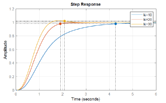 Figure \(\PageIndex{1}\): tep response of the mass-spring-damper system with integrator in the loop.
The state variable model of a DC motor is given as:
\[\frac{\rm d}{\rm dt} \left[\begin{array}{c} {i_a } \\ {\omega } \end{array}\right]=\left[\begin{array}{cc} {-100} & {-5} \\ {5} & {-10} \end{array}\right]\left[\begin{array}{c} {i_a} \\ {\omega } \end{array}\right]+\left[\begin{array}{c} {100} \\ {0} \end{array}\right]V_a , \;\;\omega =\left[\begin{array}{cc} {0} & {1} \end{array}\right]\left[\begin{array}{c} {i_a } \\ {\omega } \end{array}\right] \nonumber \]
Assume that design specifications call for a low overshoot to step response and a settling time, \(t_s\cong 0.1 \rm s\).
The control law for the tracking PI controller is given as: \(u=-k_{1} i_{a} -k_{2} \omega +k_{i} \int (r-\omega )\rm dt\).
The augmented system model for pole placement using integral control is obtained as:
\[\frac{\rm d}{\rm dt} \left[\begin{array}{c} {i_a } \\ {\omega } \\ {x_a } \end{array}\right]=\left[\begin{array}{ccc} {-100} & {-5} & {0} \\ {5} & {-10} & {0} \\ {0} & {-1} & {0} \end{array}\right]\left[\begin{array}{c} {i_a } \\ {\omega } \\ {x_a } \end{array}\right]+\left[\begin{array}{c} {100} \\ {0} \\ {0} \end{array}\right]u+\left[\begin{array}{c} {0} \\ {0} \\ {1} \end{array}\right]r \nonumber \]
The resulting characteristic polynomial is given as:
\[\Delta (s)=s^{3} +\left(100k_{1} +100\right)s^{2} +\left(1000k_{1} +500k_{2} +1025\right)s-500k_{i} . \nonumber \]
We choose a desired characteristic polynomial as: \({\mathit{\Delta}}_{des}\left(s\right)=\left(s+50\right)\left(s^2+100s+5,000\right)\). The closed-loop roots are located at: \(s=\; -50,\; -50\pm j50\).
The tracking controller is defined as: \(V_a\left(s\right)=-0.4\,i_a(t)-17.2\,\omega (t)+500\int (r-\omega )dt\).
For comparison a cascade PI controller for the transfer function model of the DC motor is designed for \(\zeta=0.7\). The PI controller is given as: \(K(s)=\frac{10(s+10)}{s}\). The closed-loop roots are placed at: \(s=-9.94, -50\pm j50.3\).
The step response of the closed-loop system for the tracking and cascade PI controllers is shown in Fig. 9.3.2. Both controllers achieve the desired settling time.
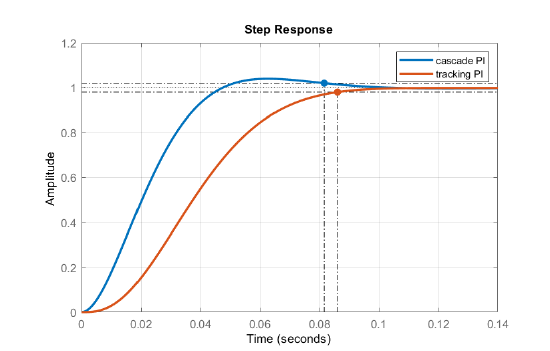
Figure \(\PageIndex{2}\): The step response of the DC motor model for cascade and tracking PI controllers.