1.3: Second-Order ODE Models

 

A physical system that contains two energy storage elements is described by a second-order ODE. Examples of second-order models are discussed below:

Example \(\PageIndex{1}\)

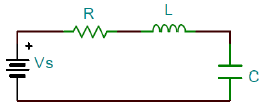
A series RLC circuit with voltage input \(V_s(t)\) and current output \(i(t)\) has a governing relationship obtained by applying the Kirchoff’s voltage law to the mesh (Figure \(\PageIndex{1}\)):

\[ L\frac{ di(t)}{ dt} +Ri(t)+\frac{1}{C} \int i(t) dt=V_ s (t) \nonumber \]

The above integro-differential equation can by converted into a second-order ODE by expressing it in terms of the electric charge, \(q(t)\), as:

\[ L\frac{ d^{2} q(t)}{ dt^{2} } +R\frac{ dq(t)}{ dt} +\frac{1}{C} q(t)=V_ s (t) \nonumber \]

Alternatively, the series RLC circuit can be described in terms of two first-order ODE’s involving natural variables, the current, \(i(t)\), and the capacitor voltage, \(V_c(t)\), as:

\[ L\frac{ di(t)}{ dt} +Ri(t)+V_{c} (t)=V_s (t), \ \ \ \ \ C\frac{dV_c}{dt}=i(t) \nonumber \]

Figure \(\PageIndex{1}\): A series RLC circuit driven by a constant voltage source.

Example \(\PageIndex{2}\)

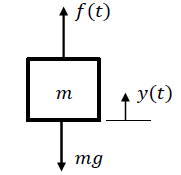
The motion of a mass element of weight, \(mg\), pulled upward by a force, \(f(t)\), is described using position output, \(y(t)\), by a second-order ODE:

\[ m\frac{ d^{2} y(t)}{ dt^{2} } +mg=f(t) \nonumber \]

The second-order ODE expresses the fact that the moving mass has both the kinetic and potential energies (Figure \(\PageIndex{2}\)).

Figure \(\PageIndex{2}\): Motion of an inertial mass under gravitational field.

Example \(\PageIndex{3}\)

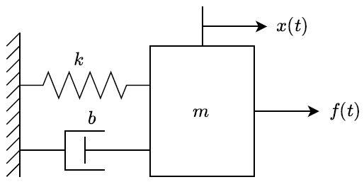
A mass–spring–damper system includes a mass affected by an applied force, \(f(t)\); its motion is restrained by a combination of a spring and a damper (Figure 1.8).

Let \(x(t)\) denote the displacement of the mass from a fixed reference; then, the dynamic equation of the system, obtained by using Newton’s second law of motion, takes a familiar form:

\[m\frac{ d^{2} x(t)}{ dt^{2} } +b\frac{ dx(t)}{ dt} +kx(t)=f(t) \nonumber \]

In compact notation, we may express the ODE as: \[m\ddot{x}\; +\; b\dot{x}\; +\; kx=f \nonumber \]

where the dots above the variable represent time derivative, i.e., \(\dot{x}\left(t\right)=\frac{dx\left(t\right)}{dt}\), \(\ddot{x}\left(t\right)=\frac{d^2x\left(t\right)}{dt^2}\).

Using position, \(x(t)\), and velocity, \(v(t)\) as variables, the mass-spring-damper system is described by two first-order equations (called state equations) given as: \[ \frac{dx}{dt}=v(t), \ \ \ \ \ \frac{dv}{dt}=\frac{1}{m} \left(-kx(t)-bv(t)+f(t) \right) \nonumber \]

In the absence of damping, the dynamic equation of the mass-spring system reduces to:

\[m\frac{d^2x\left(t\right)}{dt^2}+kx\left(t\right)=f(t) \nonumber \]

The above equation describes simple harmonic motion (SHM) with \({\omega }^2_0=k/m\). From elementary physics, the general solution to the equation is given as:

\[x\left(t\right)=A{cos {\omega }_0\ }t+B{sin {\omega }_0t\ } \nonumber \]

Figure \(\PageIndex{3}\): A mass-spring-damper system model.

Solving Second-Order Models 

A second-order ODE model can be solved by applying the Laplace transform to both sides of the differential equation. Let a general second-order ODE model be described as:

\[\ddot{y}\left(t\right)+a_1\dot{y}\left(t\right)+a_2y\left(t\right)=b_1\dot{u}\left(t\right)+b_2u\left(t\right) \nonumber \]

Application of the Laplace transform, assuming the following initial conditions: \(y\left(0\right)=y_0,\ \ \dot{y}\left(0\right)={\dot{y}}_0, \ \ u(0)=0\), gives:

\[\left(s^2+a_1s+a_2\right)y\left(s\right)-\left(s+a_1\right)y_0-{\dot{y}}_0=\left(b_1s+b_2\right)u\left(s\right) \nonumber \]

or,

\[y\left(s\right)=\frac{1}{s^2+a_1s+a_2}\left[\left(s+a_1\right)y_0+{\dot{y}}_0+\left(b_1s+b_2\right)u\left(s\right)\right] \nonumber \]

Transfer Function

By applying Laplace transform assuming no initial conditions, we obtain: \(\left(s^2+a_1s+a_2\right)y\left(s\right)=(b_1s+b_2)u(s)\); the resulting input-output transfer function is given as:

\[\frac{y\left(s\right)}{u\left(s\right)}=\frac{b_1s+b_2}{s^2+a_1s+a_2} \nonumber \]

The characteristic equation of the model is defined as: \(s^{2} +a_{1} s+a_{2} =0\).

For the mass–spring–damper model described by: \(m\ddot{x}\; +\; b\dot{x}\; +\; kx=f\)  (Example 1.3.3), the transfer function from force input to displacement output is given as:

\[\frac{x(s)}{f(s)} =\frac{1}{ms^{2} +bs+k} \nonumber \]

Transfer function of a physical systems is a proper fraction, i.e., the degree of the denominator polynomial is greater than the degree of numerator polynomial.

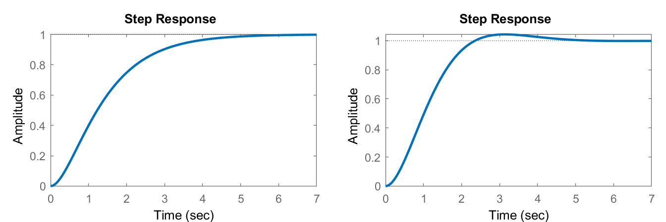
The roots of its denominator polynomial characterize the response of the second-order ODE model. The response is monotonic in the case of real roots, and oscillatory for complex roots.

Example \(\PageIndex{4}\)

Consider the mass-spring-damper model (Example \(\PageIndex{3}\)), where the following parameter values are assumed: \(m=1\), \(k=2\), and \(b=3\). Then, the second-order ODE is given as:

\[\ddot{x}\left(t\right)+3\dot{x}\left(t\right)+2x\left(t\right)=f\left(t\right) \nonumber \]

The application of the Laplace transform assuming zero initial conditions gives: \[(s^2+3s+2)y\left(s\right)=f(s) \nonumber \]

The characteristic equation of the model is given as: \(s^2+3s+2=0\). The equation has real roots at: \(s=-1,\ -2\).

Next, let \(f\left(t\right)=2u\left(t\right),\ f\left(s\right)=\frac{2}{s}\); then, the output is solved as: \[x\left(s\right)=\frac{2}{s\left(s+1\right)\left(s+2\right)} \nonumber \]

We use partial fraction expansion (PFE) to obtain:

\[x(s)=\frac{1}{s}-\frac{2}{s+1}+\frac{1}{s+2} \nonumber \]

By applying the inverse Laplace transform, the output response of the spring-mass-damper system is obtained as (Figure 1.9):

\[x\left(t\right)=\left(1-2e^{-t}+e^{-2t}\right)u(t) \nonumber \]

where \(u\left(t\right)\) represents the unit-step function.

Note: The solution of an ODE generally involves the PFE. We may use the online SimboLab partial fraction calculator for this purpose (https://www.symbolab.com/solver/part...ns-calculator/).

Example \(\PageIndex{5}\)

Consider the mass-spring-damper model (Example \(\PageIndex{3}\)), with following parameter values: \(m=1,\ k=2,\ b=2\). Then, the second-order ODE is given as:

\[\ddot{x}\left(t\right)+2\dot{x}\left(t\right)+2x\left(t\right)=f\left(t\right) \nonumber \]

The application of the Laplace transform assuming zero initial conditions gives:

\[(s^2+2s+2)y\left(s\right)=f(s) \nonumber \]

The characteristic equation of the model is given as: \(s^2+2s+2=0\). The equation has complex roots at: \(s=-1\pm j1\).

Let \(f\left(t\right)=2u\left(t\right),\ f\left(s\right)=2/s\); then, the output is solved as:

\[x\left(s\right)=\frac{2}{s\left(s^2+2s+2\right)} \nonumber \]

Next, a PFE of the output is carried out to obtain:

\[x(s)=\frac{1}{s}-\frac{s+2}{s^2+2s+2} \nonumber \]

The quadratic factor is expressed as: \({\left(s+1\right)}^2+1^2\); the quadratic term is split to obtain:

\[x\left(s\right)=\frac{1}{s}-\frac{s+1}{{\left(s+1\right)}^2+1^2}-\frac{1}{{\left(s+1\right)}^2+1^2} \nonumber \]

By applying the inverse Laplace transform, the output response of the spring-mass-damper system is obtained as (Figure 1.9):

\[x\left(t\right)=\left(1-e^{-t}\cos t -e^{-t}\sin t \right)u\left(t\right) \nonumber \]

where \(u\left(t\right)\) represents the unit-step function.

Figure \(\PageIndex{4}\): Time response of second-order system models: characteristic equation with real roots (left); with complex roots (right).

pkg load control
s=tf('s');
Gs1=1/(s^2+3*s+2);
Gs2=1/(s^2+2*s+2);
step(Gs1) 
step(Gs2)

Hello world! Hello world!