
4.4: Thévenin's Theorem
- Page ID
- 52910

\( \newcommand{\vecs}[1]{\overset { \scriptstyle \rightharpoonup} {\mathbf{#1}} } \)
\( \newcommand{\vecd}[1]{\overset{-\!-\!\rightharpoonup}{\vphantom{a}\smash {#1}}} \)
\( \newcommand{\id}{\mathrm{id}}\) \( \newcommand{\Span}{\mathrm{span}}\)
( \newcommand{\kernel}{\mathrm{null}\,}\) \( \newcommand{\range}{\mathrm{range}\,}\)
\( \newcommand{\RealPart}{\mathrm{Re}}\) \( \newcommand{\ImaginaryPart}{\mathrm{Im}}\)
\( \newcommand{\Argument}{\mathrm{Arg}}\) \( \newcommand{\norm}[1]{\| #1 \|}\)
\( \newcommand{\inner}[2]{\langle #1, #2 \rangle}\)
\( \newcommand{\Span}{\mathrm{span}}\)
\( \newcommand{\id}{\mathrm{id}}\)
\( \newcommand{\Span}{\mathrm{span}}\)
\( \newcommand{\kernel}{\mathrm{null}\,}\)
\( \newcommand{\range}{\mathrm{range}\,}\)
\( \newcommand{\RealPart}{\mathrm{Re}}\)
\( \newcommand{\ImaginaryPart}{\mathrm{Im}}\)
\( \newcommand{\Argument}{\mathrm{Arg}}\)
\( \newcommand{\norm}[1]{\| #1 \|}\)
\( \newcommand{\inner}[2]{\langle #1, #2 \rangle}\)
\( \newcommand{\Span}{\mathrm{span}}\) \( \newcommand{\AA}{\unicode[.8,0]{x212B}}\)
\( \newcommand{\vectorA}[1]{\vec{#1}} % arrow\)
\( \newcommand{\vectorAt}[1]{\vec{\text{#1}}} % arrow\)
\( \newcommand{\vectorB}[1]{\overset { \scriptstyle \rightharpoonup} {\mathbf{#1}} } \)
\( \newcommand{\vectorC}[1]{\textbf{#1}} \)
\( \newcommand{\vectorD}[1]{\overrightarrow{#1}} \)
\( \newcommand{\vectorDt}[1]{\overrightarrow{\text{#1}}} \)
\( \newcommand{\vectE}[1]{\overset{-\!-\!\rightharpoonup}{\vphantom{a}\smash{\mathbf {#1}}}} \)
\( \newcommand{\vecs}[1]{\overset { \scriptstyle \rightharpoonup} {\mathbf{#1}} } \)
\( \newcommand{\vecd}[1]{\overset{-\!-\!\rightharpoonup}{\vphantom{a}\smash {#1}}} \)
\(\newcommand{\avec}{\mathbf a}\) \(\newcommand{\bvec}{\mathbf b}\) \(\newcommand{\cvec}{\mathbf c}\) \(\newcommand{\dvec}{\mathbf d}\) \(\newcommand{\dtil}{\widetilde{\mathbf d}}\) \(\newcommand{\evec}{\mathbf e}\) \(\newcommand{\fvec}{\mathbf f}\) \(\newcommand{\nvec}{\mathbf n}\) \(\newcommand{\pvec}{\mathbf p}\) \(\newcommand{\qvec}{\mathbf q}\) \(\newcommand{\svec}{\mathbf s}\) \(\newcommand{\tvec}{\mathbf t}\) \(\newcommand{\uvec}{\mathbf u}\) \(\newcommand{\vvec}{\mathbf v}\) \(\newcommand{\wvec}{\mathbf w}\) \(\newcommand{\xvec}{\mathbf x}\) \(\newcommand{\yvec}{\mathbf y}\) \(\newcommand{\zvec}{\mathbf z}\) \(\newcommand{\rvec}{\mathbf r}\) \(\newcommand{\mvec}{\mathbf m}\) \(\newcommand{\zerovec}{\mathbf 0}\) \(\newcommand{\onevec}{\mathbf 1}\) \(\newcommand{\real}{\mathbb R}\) \(\newcommand{\twovec}[2]{\left[\begin{array}{r}#1 \\ #2 \end{array}\right]}\) \(\newcommand{\ctwovec}[2]{\left[\begin{array}{c}#1 \\ #2 \end{array}\right]}\) \(\newcommand{\threevec}[3]{\left[\begin{array}{r}#1 \\ #2 \\ #3 \end{array}\right]}\) \(\newcommand{\cthreevec}[3]{\left[\begin{array}{c}#1 \\ #2 \\ #3 \end{array}\right]}\) \(\newcommand{\fourvec}[4]{\left[\begin{array}{r}#1 \\ #2 \\ #3 \\ #4 \end{array}\right]}\) \(\newcommand{\cfourvec}[4]{\left[\begin{array}{c}#1 \\ #2 \\ #3 \\ #4 \end{array}\right]}\) \(\newcommand{\fivevec}[5]{\left[\begin{array}{r}#1 \\ #2 \\ #3 \\ #4 \\ #5 \\ \end{array}\right]}\) \(\newcommand{\cfivevec}[5]{\left[\begin{array}{c}#1 \\ #2 \\ #3 \\ #4 \\ #5 \\ \end{array}\right]}\) \(\newcommand{\mattwo}[4]{\left[\begin{array}{rr}#1 \amp #2 \\ #3 \amp #4 \\ \end{array}\right]}\) \(\newcommand{\laspan}[1]{\text{Span}\{#1\}}\) \(\newcommand{\bcal}{\cal B}\) \(\newcommand{\ccal}{\cal C}\) \(\newcommand{\scal}{\cal S}\) \(\newcommand{\wcal}{\cal W}\) \(\newcommand{\ecal}{\cal E}\) \(\newcommand{\coords}[2]{\left\{#1\right\}_{#2}}\) \(\newcommand{\gray}[1]{\color{gray}{#1}}\) \(\newcommand{\lgray}[1]{\color{lightgray}{#1}}\) \(\newcommand{\rank}{\operatorname{rank}}\) \(\newcommand{\row}{\text{Row}}\) \(\newcommand{\col}{\text{Col}}\) \(\renewcommand{\row}{\text{Row}}\) \(\newcommand{\nul}{\text{Nul}}\) \(\newcommand{\var}{\text{Var}}\) \(\newcommand{\corr}{\text{corr}}\) \(\newcommand{\len}[1]{\left|#1\right|}\) \(\newcommand{\bbar}{\overline{\bvec}}\) \(\newcommand{\bhat}{\widehat{\bvec}}\) \(\newcommand{\bperp}{\bvec^\perp}\) \(\newcommand{\xhat}{\widehat{\xvec}}\) \(\newcommand{\vhat}{\widehat{\vvec}}\) \(\newcommand{\uhat}{\widehat{\uvec}}\) \(\newcommand{\what}{\widehat{\wvec}}\) \(\newcommand{\Sighat}{\widehat{\Sigma}}\) \(\newcommand{\lt}{<}\) \(\newcommand{\gt}{>}\) \(\newcommand{\amp}{&}\) \(\definecolor{fillinmathshade}{gray}{0.9}\)Thévenin's theorem, named after Léon Charles Thévenin, is a powerful analysis tool. For DC, it states:
\[\text{Any single port linear network can be reduced to a simple voltage source, } E_{th}, \text{in series with an internal resistance, } R_{th}. \nonumber \]
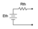
Figure 6.4.1 : Thévenin equivalent circuit.
An example is shown in Figure 6.4.1 . The phrase “single port network” means that the circuit is cut in such a way that only two connections exist to the remainder of the circuit (two connection points makes up one port). The remainder of the circuit may be a single component or a large multi-component sub-circuit. As there are many ways to cut a typical circuit, there are many possible Thévenin equivalents. The important thing is that there are only two connection points between the two portions of the circuit and neither point has to be ground.
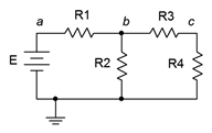
Figure 6.4.2 : Example circuit.
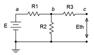
Figure 6.4.3 : Finding \(E_{th}\)..
Consider the circuit shown in Figure 6.4.2 . Suppose we cut the circuit immediately to the left of \(R_4\). That is, we will find the Thévenin equivalent that drives \(R_4\). The first step is to make the cut, removing the remainder of the circuit (in this case, just \(R_4\)). We then determine the open circuit output voltage. This is the maximum voltage that could appear between the cut points and is called the Thévenin voltage, \(E_{th}\). This is shown in Figure 6.4.3 . In a circuit such as this, basic series-parallel analysis may be used to find \(E_{th}\). This process turns out to be quite straightforward in this particular circuit. Due to the open, no current flows through \(R_3\), thus no voltage is developed across \(R_3\), and therefore \(E_{th}\) must equal the voltage developed across \(R_2\) which may be obtained via a voltage divider with resistor \(R_1\) and source \(E\).
The second part is finding the Thévenin resistance, \(R_{th}\). Beginning with the “cut” circuit, replace all sources with their ideal internal resistance (thus shorting voltage sources and opening current sources). From the perspective of the cut point, look back into the circuit and simplify by making appropriate series and parallel combinations to determine its equivalent resistance. This is shown in Figure 6.4.4 . Looking in from where the cut was made (right-to-left here), we find that \(R_1\) and \(R_2\) are in parallel, and this combination is then in series with \(R_3\). Thus, \(R_{th} = R_3 + (R_1 || R_2)\). A common error is to determine the equivalent resistance that the source drives. Remember, everything is determined from the vantage point of the cut or port.
Thévenin equivalents are not limited to single source circuits. It is possible to find the equivalent of a network with several sources. Finding the open circuit output voltage will undoubtedly require some extra work, for example the use of superposition of source conversions. Finding the Thévenin resistance is unchanged, just remember to replace every source with its ideal internal resistance before simplifying the network.
As noted earlier, the original circuit could be cut in a number of different ways. We might, for example, want to determine the Thévenin equivalent that drives \(R_2\) in the circuit of Figure 6.4.2 . This cut appears in Figure 6.4.5 . Clearly, this will result in different values for both \(E_{th}\) and \(R_{th}\). For example, \(R_{th}\) is now \(R_1 || (R_3 + R_4)\).
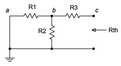
Figure 6.4.4 : Finding \(R_{th}\).
Finding Thévenin Equivalents in Lab
The procedure for experimentally determining an equivalent in the laboratory mimics the analytical approach. The first step is to figuratively cut the circuit and isolate the section that is to be converted. At this point we have the open circuit version of the circuit and all we need do is connect a multimeter to the open port to determine \(E_{th}\).
There are two methods for determining \(R_{th}\). The first method works well for simple circuits that use only resistors and current and/or voltage sources. The second method is more generally applicable and will work for circuits with active devices such as transistors. To use the first method, the sources are physically removed from the circuit and replaced with their ideal internal resistance. Thus voltage sources are replaced with a shorting wire and current sources are left as opens. Do not simply place shorting wires across the terminals of voltage sources as doing so will cause an overload and potentially damage the sources. Once this is completed, a multimeter is placed at the open port and set to read resistance. The indicated value is \(R_{th}\).
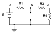
Figure 6.4.5 : An alternate cut or port location.
The second method uses a variable resistance, namely either a rheostat or a decade box, and exploits the voltage divider rule. In this version, the sources are left active (powered up) and are not replaced with opens or shorts. Once \(E_{th}\) is measured, the variable resistor is placed across the port connections. This resistance is adjusted until the port voltage drops to exactly half of \(E_{th}\). In the equivalent circuit, there are only two resistances of concern, \(R_{th}\) and this variable load resistance, and they are in series. Consequently, if the load voltage is now half of the open circuit voltage (\(E_{th}\)), then the other half of the voltage must be dropping across the equivalent internal resistance (\(R_{th}\)). For this to be true in a series circuit, the two resistances must have the same value. Thus, we simply remove the rheostat from the circuit and use a multimeter to determine its precise value. If a decade box is used instead, the value is determined directly by reading the knob settings.
Whether determined analytically or empirically, the Thévenin equivalent circuit can replace the original single port network regardless of what the original was connected to. The same voltages and currents will be seen in this other portion, and it won't matter if the other portion is comprised of a single resistor, multiple resistors, multiple resistors and multiple sources, or even multiple resistors and sources wired to a selection of piquant cheeses. The Thévenin equivalent is a true functional equivalent and can be used on any linear bilateral network.
Determine the Thévenin equivalent of the circuit driving the 1 k\(\Omega\) in Figure 6.4.6 . Verify that the equivalent produces the same voltage across this resistor as the original circuit.
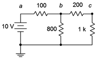
Figure 6.4.6 : Circuit for Example 6.4.1 .
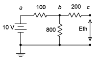
Figure 6.4.7 : Finding \(E_{th}\).
First, we'll redraw the circuit showing the portion to be Théveninized, as shown in Figure 6.4.7 . The open circuit output voltage will be the voltage across the 800 \(\Omega\) resistor as there will be no voltage drop across the 200 \(\Omega\) resistor (as no current flows through it into the open). This is found via a simple voltage divider.
\[E_{th} = E \frac{R_x}{R_x+R_y} \nonumber \]
\[E_{th} = 10 V \frac{800 \Omega}{800\Omega +100 \Omega} \nonumber \]
\[E_{th} \approx 8.889 V \nonumber \]
The equivalent resistance is found by shorting the voltage source and then simplifying the circuit. The result is 200 \(\Omega\) in series with the parallel combination of the 100 \(\Omega\) and 800 \(\Omega\). \(200 + 100 || 800 \approx 288.89 \Omega\).
To determine Vc, we can use a voltage divider between the 1 k\(\Omega\) and the 288.89 \(\Omega\) along with the equivalent source voltage of 8.889 volts.
\[V_c = E_{th} \frac{R_L}{R_L+R_{th}} \nonumber \]
\[V_c = 8.889V \frac{1k \Omega}{ 1 k\Omega +288.89\Omega} \nonumber \]
\[V_c \approx 6.897V \nonumber \]
Now let's determine \(V_c\) in the original circuit using series-parallel analysis techniques. Perhaps the quickest approach is a pair of voltage dividers. \(V_b\) is found via a divider between the parallel combination of the 1 k\(\Omega\) + 200 \(\Omega\) and the 800 \(\Omega\), against the 100 \(\Omega\). \(V_c\) is is then found using that voltage with a divider between the 1 k\(\Omega\) and 200 \(\Omega\). Using this approach, \(V_b\) is approximately 8.276 volts and \(V_c\) is approximately 6.897 volts, providing an excellent match.
It might seem that the Thévenin method is the “long way home” in this example, and it is, but it has the advantage of being more efficient if several different loads are being considered. For example, suppose we decided to determine the output voltage not just for the 1 k\(\Omega\), but for a group of a half dozen different resistors. The double voltage divider would have to be determined for each load resistor using the straight series-parallel method but only a single divider needs to be computed for each load when using the Thévenin method. The Thévenin method is also of great use when determining maximum power transfer, as we shall see a later in this chapter.
Computer Simulation
To verify the results of Example 6.4.1 , the original circuit is recreated in a simulator along its Thévenin equivalent, as shown in Figure 6.4.8 .
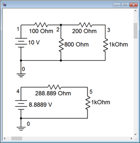
Figure 6.4.8 : The original circuit of Example 6.4.1 in a simulator along with the equivalent.
A DC operating point analysis is performed and the results are shown in Figure 6.4.9 . Note that the voltages across the identical 1 k\(\Omega\) loads (nodes 3 and 5) are virtually the same, indicating functional equivalence between the two. The slight deviation is due to the rounding of the Thévenin voltage and resistance.
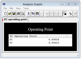
Figure 6.4.9 : Results of the simulation showing equivalence.
As a further check, the simulation is run again, but this time using an alternate load resistor value. The value chosen is the Thévenin resistance value. By matching the resistances, this should produce a 50/50 voltage divider and the load voltage should equal half of the Thévenin source voltage, or approximately 4.444 volts. That is precisely what we find, as seen in Figure 6.4.10 .
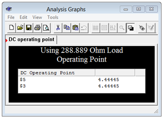
Figure 6.4.10 : Results of the simulation for matched resistance.
As mentioned previously, Thévenin's theorem can be applied to much more complex multi-source circuits, and the item being driven need not be just a single resistor. This is illustrated in the next example.
Determine the Thévenin equivalent of the circuit driving the resistor/voltage source combo in Figure 6.4.11 . Verify that the equivalent produces the same voltage across this resistor as the original circuit.
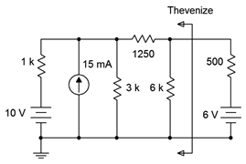
Figure 6.4.11 : Circuit for Example 6.4.2 .
Determining \(R_{th}\) is not particularly difficult here. After shorting the 10 volt source and open the current source, it can be seen that the 1 k\(\Omega\) and 3 k\(\Omega\) are in parallel, yielding 750 \(\Omega\). This is in series with the 1250 \(\Omega\) for a total of 2 k\(\Omega\), which is in turn in parallel with the 6 k\(\Omega\). The final result is 1.5 k\(\Omega\).
Finding \(E_{th}\) is a little more involved. One possibility is to use a source conversion on the 10 volt source as that will leave us with two parallel current sources that may be combined directly. The converted source will be 10 V/ 1k\(\Omega\), or 10 mA, in parallel with 1 k\(\Omega\). This results in a total of 25 mA feeding upwards with 1 k\(\Omega\) \(||\) 3 k\(\Omega\), or 750 \(\Omega\). We can use the current divider rule to determine the current flowing through the 1250 \(\Omega\) plus 6 k\(\Omega\) branch, and then use Ohm's law to find the open circuit voltage (i.e., the voltage across the 6 k\(\Omega\)).
\[I_{6k} = I_S \frac{R_x}{R_x+R_y} \nonumber \]
\[I_{6k} = 25 mA \frac{750\Omega}{ 750\Omega +7250\Omega} \nonumber \]
\[I_{6k} = 2.34375 mA \nonumber \]
\[E_{th} = I_{6k} \times R_{6k} \nonumber \]
\[E_{th} = 2.34375 mA \times 6 k \Omega \nonumber \]
\[E_{th} = 14.0625V \nonumber \]
Another approach to determine this value would be to use superposition. This is left as an additional exercise.
Turning our attention to the voltage produced across the 6 volt with 500 \(\Omega\) sub-circuit, we have a simple series loop with \(E_{th}\) opposing this 6 volt source, leaving 8.0625 volts to produce a clockwise current through \(R_{th}\) in series with the 500 \(\Omega\) (a total of 2 k\(\Omega\)). That current will be 8.0625 V / 2 k\(\Omega\), or 4.03125 mA. This will produce a drop across the 500 \(\Omega\) of 2.015625 volts with a polarity of + to − from top to bottom. This will add to the 6 volt source resulting in a final potential of 8.015625 volts. The results are verified via the simulation technique used previously. The node voltages for both the original and equivalent circuits are shown in Figure 6.4.12 .
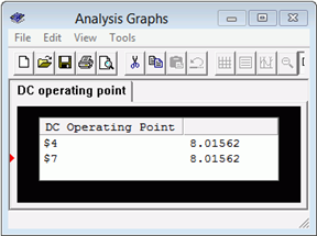
Figure 6.4.12 : Results of the simulation using the original and equivalent circuits.