
12.4: Thévenin's and Norton's Theorems
- Page ID
- 52971

\( \newcommand{\vecs}[1]{\overset { \scriptstyle \rightharpoonup} {\mathbf{#1}} } \)
\( \newcommand{\vecd}[1]{\overset{-\!-\!\rightharpoonup}{\vphantom{a}\smash {#1}}} \)
\( \newcommand{\id}{\mathrm{id}}\) \( \newcommand{\Span}{\mathrm{span}}\)
( \newcommand{\kernel}{\mathrm{null}\,}\) \( \newcommand{\range}{\mathrm{range}\,}\)
\( \newcommand{\RealPart}{\mathrm{Re}}\) \( \newcommand{\ImaginaryPart}{\mathrm{Im}}\)
\( \newcommand{\Argument}{\mathrm{Arg}}\) \( \newcommand{\norm}[1]{\| #1 \|}\)
\( \newcommand{\inner}[2]{\langle #1, #2 \rangle}\)
\( \newcommand{\Span}{\mathrm{span}}\)
\( \newcommand{\id}{\mathrm{id}}\)
\( \newcommand{\Span}{\mathrm{span}}\)
\( \newcommand{\kernel}{\mathrm{null}\,}\)
\( \newcommand{\range}{\mathrm{range}\,}\)
\( \newcommand{\RealPart}{\mathrm{Re}}\)
\( \newcommand{\ImaginaryPart}{\mathrm{Im}}\)
\( \newcommand{\Argument}{\mathrm{Arg}}\)
\( \newcommand{\norm}[1]{\| #1 \|}\)
\( \newcommand{\inner}[2]{\langle #1, #2 \rangle}\)
\( \newcommand{\Span}{\mathrm{span}}\) \( \newcommand{\AA}{\unicode[.8,0]{x212B}}\)
\( \newcommand{\vectorA}[1]{\vec{#1}} % arrow\)
\( \newcommand{\vectorAt}[1]{\vec{\text{#1}}} % arrow\)
\( \newcommand{\vectorB}[1]{\overset { \scriptstyle \rightharpoonup} {\mathbf{#1}} } \)
\( \newcommand{\vectorC}[1]{\textbf{#1}} \)
\( \newcommand{\vectorD}[1]{\overrightarrow{#1}} \)
\( \newcommand{\vectorDt}[1]{\overrightarrow{\text{#1}}} \)
\( \newcommand{\vectE}[1]{\overset{-\!-\!\rightharpoonup}{\vphantom{a}\smash{\mathbf {#1}}}} \)
\( \newcommand{\vecs}[1]{\overset { \scriptstyle \rightharpoonup} {\mathbf{#1}} } \)
\( \newcommand{\vecd}[1]{\overset{-\!-\!\rightharpoonup}{\vphantom{a}\smash {#1}}} \)
\(\newcommand{\avec}{\mathbf a}\) \(\newcommand{\bvec}{\mathbf b}\) \(\newcommand{\cvec}{\mathbf c}\) \(\newcommand{\dvec}{\mathbf d}\) \(\newcommand{\dtil}{\widetilde{\mathbf d}}\) \(\newcommand{\evec}{\mathbf e}\) \(\newcommand{\fvec}{\mathbf f}\) \(\newcommand{\nvec}{\mathbf n}\) \(\newcommand{\pvec}{\mathbf p}\) \(\newcommand{\qvec}{\mathbf q}\) \(\newcommand{\svec}{\mathbf s}\) \(\newcommand{\tvec}{\mathbf t}\) \(\newcommand{\uvec}{\mathbf u}\) \(\newcommand{\vvec}{\mathbf v}\) \(\newcommand{\wvec}{\mathbf w}\) \(\newcommand{\xvec}{\mathbf x}\) \(\newcommand{\yvec}{\mathbf y}\) \(\newcommand{\zvec}{\mathbf z}\) \(\newcommand{\rvec}{\mathbf r}\) \(\newcommand{\mvec}{\mathbf m}\) \(\newcommand{\zerovec}{\mathbf 0}\) \(\newcommand{\onevec}{\mathbf 1}\) \(\newcommand{\real}{\mathbb R}\) \(\newcommand{\twovec}[2]{\left[\begin{array}{r}#1 \\ #2 \end{array}\right]}\) \(\newcommand{\ctwovec}[2]{\left[\begin{array}{c}#1 \\ #2 \end{array}\right]}\) \(\newcommand{\threevec}[3]{\left[\begin{array}{r}#1 \\ #2 \\ #3 \end{array}\right]}\) \(\newcommand{\cthreevec}[3]{\left[\begin{array}{c}#1 \\ #2 \\ #3 \end{array}\right]}\) \(\newcommand{\fourvec}[4]{\left[\begin{array}{r}#1 \\ #2 \\ #3 \\ #4 \end{array}\right]}\) \(\newcommand{\cfourvec}[4]{\left[\begin{array}{c}#1 \\ #2 \\ #3 \\ #4 \end{array}\right]}\) \(\newcommand{\fivevec}[5]{\left[\begin{array}{r}#1 \\ #2 \\ #3 \\ #4 \\ #5 \\ \end{array}\right]}\) \(\newcommand{\cfivevec}[5]{\left[\begin{array}{c}#1 \\ #2 \\ #3 \\ #4 \\ #5 \\ \end{array}\right]}\) \(\newcommand{\mattwo}[4]{\left[\begin{array}{rr}#1 \amp #2 \\ #3 \amp #4 \\ \end{array}\right]}\) \(\newcommand{\laspan}[1]{\text{Span}\{#1\}}\) \(\newcommand{\bcal}{\cal B}\) \(\newcommand{\ccal}{\cal C}\) \(\newcommand{\scal}{\cal S}\) \(\newcommand{\wcal}{\cal W}\) \(\newcommand{\ecal}{\cal E}\) \(\newcommand{\coords}[2]{\left\{#1\right\}_{#2}}\) \(\newcommand{\gray}[1]{\color{gray}{#1}}\) \(\newcommand{\lgray}[1]{\color{lightgray}{#1}}\) \(\newcommand{\rank}{\operatorname{rank}}\) \(\newcommand{\row}{\text{Row}}\) \(\newcommand{\col}{\text{Col}}\) \(\renewcommand{\row}{\text{Row}}\) \(\newcommand{\nul}{\text{Nul}}\) \(\newcommand{\var}{\text{Var}}\) \(\newcommand{\corr}{\text{corr}}\) \(\newcommand{\len}[1]{\left|#1\right|}\) \(\newcommand{\bbar}{\overline{\bvec}}\) \(\newcommand{\bhat}{\widehat{\bvec}}\) \(\newcommand{\bperp}{\bvec^\perp}\) \(\newcommand{\xhat}{\widehat{\xvec}}\) \(\newcommand{\vhat}{\widehat{\vvec}}\) \(\newcommand{\uhat}{\widehat{\uvec}}\) \(\newcommand{\what}{\widehat{\wvec}}\) \(\newcommand{\Sighat}{\widehat{\Sigma}}\) \(\newcommand{\lt}{<}\) \(\newcommand{\gt}{>}\) \(\newcommand{\amp}{&}\) \(\definecolor{fillinmathshade}{gray}{0.9}\)These theorems are related in that they allow complex linear networks to be simplified down to a single source with an associated internal impedance. They simplify analysis when checking a circuit with multiple possible loads.
Thévenin's Theorem
Thévenin's theorem is named after Léon Charles Thévenin. It states that:
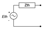
\[\text{Any single port linear network can be reduced to a simple voltage source, } E_{th}, \text{ in series with an internal impedance } Z_{th}. \nonumber \]
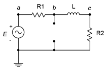
It is important to note that a Thévenin equivalent is valid only at a particular frequency. If the system frequency is changed, the reactance and impedance values will change and the resulting \(E_{th}\) and \(Z_{th}\) values will be altered. Consequently, these equivalents are generally not appropriate for a circuit using multiple sources with differing frequencies1. A generic example of a Thévenin equivalent is shown in Figure \(\PageIndex{1}\).
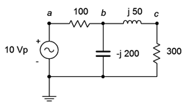
The phrase “single port network” means that the original circuit is cut in such a way that only two connections exist to the remainder of the circuit. That remainder may be a single component or a large multi-component sub-circuit. \(E_{th}\) is the open circuit voltage at the port and \(Z_{th}\) is the impedance looking back into the port (i.e., the equivalent that now drives the remainder). As there are many ways to cut a typical circuit, there are many possible Thévenin equivalents. Consider the circuit shown in Figure \(\PageIndex{2}\).
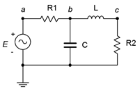
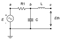
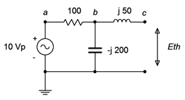
Suppose we want to find the Thévenin equivalent that drives \(R_2\). We cut the circuit immediately to the left of \(R_2\). That is, The first step is to make the cut, removing the remainder of the circuit. In this case the remainder is just \(R_2\). We then determine the open circuit output voltage at the cut points (i.e., at the open port). This voltage is called the Thévenin voltage, \(E_{th}\). This is shown in Figure \(\PageIndex{3}\). In a circuit such as this, basic series-parallel analysis techniques may be used to find \(E_{th}\). In this circuit, due to the open, no current flows through the inductor, \(L\), and thus no voltage is developed across it. Therefore, \(E_{th}\) must equal the voltage developed across the capacitor, \(C\).
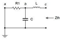
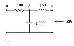
The second part is finding the Thévenin impedance, \(Z_{th}\). Beginning with the “cut” circuit, replace all sources with their ideal internal impedance (thus shorting voltage sources and opening current sources). From the perspective of the cut point, look back into the circuit and simplify to determine its equivalent impedance. This is shown in Figure \(\PageIndex{4}\). Looking in from where the cut was made (right side), we see that \(R_1\) and \(X_C\) are in parallel, and this combination is then in series with \(X_L\). Thus, \(Z_{th}\) is equal to \(jX_L + (R1 || −jX_C)\).
As noted earlier, the original circuit could be cut in a number of different ways. We might, for example, want to determine the Thévenin equivalent that drives \(C\) in the original circuit of Figure \(\PageIndex{2}\). The new port location appears in Figure \(\PageIndex{5}\).
Clearly, this will result in different values for both \(E_{th}\) and \(Z_{th}\). For example, \(Z_{th}\) is now \(R_1 || (R_2 + jX_L)\).
A common error is to find \(Z_{th}\) from the wrong perspective, namely, finding the impedance that the source drives. This is flatly incorrect. Remember, \(Z_{th}\) is found by looking into the port and simplifying whatever is seen from there. One way to remember this is that it is possible to create equivalents for multi-source circuits. In that instance, there isn't a single driving source, so finding its load impedance is nonsensical.
Measuring the Thévenin Equivalent in the Laboratory
In a laboratory situation, the Thévenin equivalent can be found quickly and efficiently with the proper tools. First, the circuit is “cut”, leaving just the portion to be Thévenized. The voltage at the cut points is measured with an oscilloscope. This is \(E_{th}\). All of the sources are then replaced with their internal impedance, ideally shorting voltage sources and opening current sources2. An LCR impedance meter can then be connected to the port to read \(Z_{th}\). If an impedance meter is not available, then the source(s) are left in place and an LCR substitution box is placed at the cut points. The box is adjusted so that the voltage across it is equal to half of \(E_{th}\). By the voltage divider rule, the value of the substitution box must be equal to \(Z_{th}\). In this case, the substitution box will yield either an inductance or capacitance value which can then be turned into a reactance given the frequency.
Example \(\PageIndex{1}\)
For the circuit of Figure \(\PageIndex{6}\), determine the Thévenin equivalent that drives the 300 \(\Omega\) resistor and find \(v_c\). Assume the source angle is \(0^{\circ}\).
First, let's find \(E_{th}\), the open circuit output voltage. We cut the circuit so that the 300 \(\Omega\) resistor is removed. Then we determine the voltage at the cut points. This circuit is shown in Figure \(\PageIndex{7}\).
There is no current flowing through the inductor due to the open. Therefore, the voltage across the inductor is zero. Consequently, \(E_{th}\) is the voltage across the capacitor, and that can be found with a voltage divider.
\[E_{th} = E \frac{X_C}{X_C +R_1} \nonumber \]
\[E_{th} = 10 \angle 0^{\circ} V \frac{− j 200\Omega}{− j 200\Omega +100 \Omega} \nonumber \]
\[E_{th} = 8.944\angle −26.6^{\circ} V \text{ or } 8 − j 4 V \nonumber \]
To find \(Z_{th}\), we replace the source with a short and then look back in from the cut points. The equivalent circuit is shown in Figure \(\PageIndex{8}\). The inductor is in series with the parallel combination of the resistor and capacitor.
\[Z_{left2} = \frac{R \times jX_C}{R − jX_C} \nonumber \]
\[Z_{left2} = \frac{100 \Omega \times (− j 200 \Omega )}{100 \Omega − j 200 \Omega} \nonumber \]
\[Z_{left2} = 89.44\angle −26.6^{\circ} \Omega \nonumber \]
\[Z_{th} = Z_{left2} + X_L \nonumber \]
\[Z_{th} = 89.44\angle −26.6 ^{\circ} \Omega + j 50\Omega \nonumber \]
\[Z_{th} = 80.62\angle 7.12^{\circ} \Omega or 80 +j 10\Omega \nonumber \]
The completed equivalent is shown in Figure \(\PageIndex{9}\).
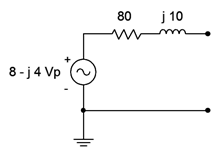
The voltage across the 300 \(\Omega\) resistor can be found directly:
\[v_{R2} = E_{th} \frac{R_2}{Z_{th} + R_2} \nonumber \]
\[v_{R2} = 8 − j 4 V \frac{300\Omega}{80+j 10\Omega +300\Omega} \nonumber \]
\[v_{R2} = 7.06\angle −28.1^{\circ} V \nonumber \]
This value can be verified by following a standard series-parallel simplification. For example, the impedance of the three rightmost components \((181.4\angle −53.97^{\circ} \Omega )\) forms a voltage divider with the 100 \(\Omega\) resistor and the 10 volt source. This leads to \(v_b\) \((7.156\angle −18.61^{\circ}\) volts ). A second divider can then be used between \(v_b\), the inductor and the 300 \(\Omega\) resistor to find \(v_c\), which is \(7.06\angle −28.1^{\circ}\) volts as expected. The big advantage of using the Thévenin equivalent is that we can easily find \(v_c\) for any other value of load because we need only analyze the simpler equivalent circuit rather than the original.
Thévenin's theorem can also be used on multi-source circuits. The technique for finding \(Z_{th}\) does not change, however, finding \(E_{th}\) is a little more involved, as illustrated in the next example.
Example \(\PageIndex{2}\)
Find \(v_b\) for the circuit of Figure \(\PageIndex{10}\) using Thévenin's theorem.
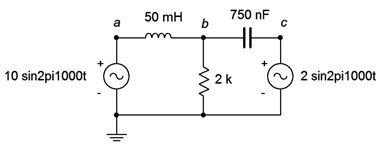
This circuit is similar to the one used in Example 5.3.2 (Figure 5.3.5). The difference here is that the second source uses the same frequency as the first source. The reactance values are:
\[X_L = j314.2 \Omega \nonumber \]
\[X_C = −j212.2 \Omega \nonumber \]
The voltage across the 2 k\(\Omega\) is \(v_b\), so we'll treat that resistor as the load in order to define the equivalent circuit. This is redrawn in Figure \(\PageIndex{11}\).
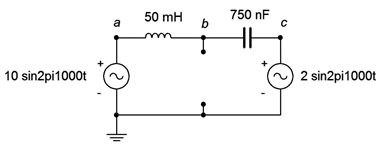
To find \(Z_{th}\), we short the two sources. We're left with the inductor and capacitor in parallel. If this is confusing, remember that we are looking from node \(b\) to ground (the cut points), so they are not in series. That is, if a sensing current entered at node \(b\), it could split left and right, indicating parallel paths, not a series connection.
\[Z_{th} = \frac{− jX_C \times jX_L}{− jX_C +jX_L} \nonumber \]
\[Z_{th} = \frac{− j 212.2\Omega \times j 314.2 \Omega}{− j 212.2 \Omega + j 314.2 \Omega} \nonumber \]
\[Z_{th} = − j 653.7\Omega \nonumber \]
We have a few options to find \(E_{th}\). Superposition could be used, each circuit requiring a voltage divider. Alternately, the equivalent is basically a series loop as far as finding \(v_b\) is concerned. Thus, we could find the voltage across the inductor and subtract that from the left source (assuming a reference current direction of clockwise). Finding the inductor voltage requires either a voltage divider or finding the current. Neither approach is considerably less work than the other, and it's probably a good idea to get in a little more practice using superposition, so...
Considering the left source, we short the right source and find \(v_b\).
\[v_{bR} = E_1 \frac{X_C}{X_C +X_L} \nonumber \]
\[v_{bR} = 10 \angle 0^{\circ} V \frac{−j 212.2\Omega}{− j 212.2\Omega +j 314.2 \Omega} \nonumber \]
\[v_{bR} = 20.84\angle 180 ^{\circ} V \text{ or } −20.84\angle 0^{\circ} V \nonumber \]
For the right source, we short the left source and find \(v_b\). Then we add the two contributions to find the final voltage. Note that both sources will produce a reference polarity of + to − from top to bottom.
\[v_{bL} = E_2 \frac{X_C}{X_C + X_L} \nonumber \]
\[v_{bL} = 2\angle 0^{\circ} V \frac{j 314.2\Omega}{− j 212.2 \Omega +j 314.2 \Omega} \nonumber \]
\[v_{bL} = 6.16\angle 0^{\circ} V \nonumber \]
The sum of the two is \(−20.84\angle 0^{\circ} + 6.16\angle 0^{\circ}\), or \(14.68\angle 180^{\circ}\) volts. The Thévenin equivalent is a source of \(14.68\angle 180^{\circ}\) volts in series with an impedance of \(−j653.7 \Omega \).
To find the voltage across the 2 k\(\Omega\) resistor, we apply it to the equivalent circuit and solve.
\[v_b = E_{th} \frac{R}{R +Z_{th}} \nonumber \]
\[v_b = 14.68\angle 180 ^{\circ} V \frac{2 k\Omega}{ 2k \Omega +(− j 653.7\Omega )} \nonumber \]
\[v_b = 13.95\angle −161.9^{\circ} V \nonumber \]
Computer Simulation
To verify the results of the preceding example, the circuit of Figure \(\PageIndex{10}\) is captured in a simulator, as shown in Figure \(\PageIndex{12}\).
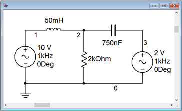
Next, a transient analysis is run, plotting the voltage at node 2, which corresponds to \(v_b\) in the original circuit. The result is shown in Figure \(\PageIndex{13}\). The plot is delayed by 0.1 seconds in order to get past the initial turn-on transient.
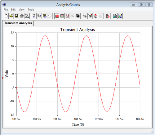
Both the amplitude and phase of the simulation waveform match the computed results.
Norton's Theorem
Norton's theorem is named after Edward Lawry Norton. It is the current source version of Thévenin's theorem. In other words, complex networks can be reduced to a single current source with a parallel internal impedance. Formally, Norton's theorem states:
\[\text{Any single port linear network can be reduced to a simple voltage source, } I_n, \text{ in parallel with an internal impedance } Z_n. \nonumber \]
The process of finding a Norton equivalent is very similar to finding a Thévenin equivalent. First, the Norton impedance is the same as the Thévenin impedance. Second, instead of finding the open circuit output voltage, the short circuit output current is found. This is the Norton current. Due to the equivalence afforded by source conversions, if a Thévenin equivalent for a network can be created, then it must be possible to create a Norton equivalent. Indeed, if a Thévenin equivalent is found, a source conversion can be performed on it to yield the Norton equivalent.
Example \(\PageIndex{3}\)
Let's reexamine Example \(\PageIndex{1}\), this time creating a Norton equivalent circuit. For convenience, the original circuit of Figure \(\PageIndex{6}\) is repeated in Figure \(\PageIndex{14}\). Once again, the goal will be to determine the equivalent that drives the 300 \(\Omega\) resistor and to find vc.

As noted, the Norton impedance, \(Z_n\), is the same as \(Z_{th}\). That was \(80 + j10 \Omega \). The Norton current, \(I_n\), is the short-circuit current through the cut points. We can think of this as replacing the load resistor with an ammeter. This is the same as the current through the inductor. In this situation, the capacitor and inductor are in parallel and yield an impedance of \(j66.67 \Omega \). Thus, the source current is:
\[i_{source} = \frac{E}{R +Z_{LC}} \nonumber \]
\[i_{source} = \frac{10\angle 0^{\circ}}{100\Omega +j 66.67\Omega} \nonumber \]
\[i_{source} = 83.2E-3\angle −33.7^{\circ} A \nonumber \]
This splits between the capacitor and inductor. Using the current divider rule we find:
\[i_n = i_{inductor} = I_{source} \frac{X_C}{X_C+X_L} \nonumber \]
\[i_n = 83.2 \angle −33.7^{\circ} A \frac{− j 200\Omega}{− j 200 \Omega +j 50\Omega} \nonumber \]
\[i_n = 0.1109\angle −33.7 ^{\circ} A \nonumber \]
A source conversion can be applied to verify this value. The resulting voltage source is \(8 − j4\) volts, precisely the value of the Thévenin equivalent.
Ultimately, deciding between using the Thévenin or Norton equivalents is a matter of personal taste and convenience. They work equally well.
References
1It is possible that an equivalent can be valid across a specified range of frequencies, but it will not hold for all frequencies.
2A typical laboratory signal generator has a 50 \(\Omega\) internal impedance, and using this value would be more accurate than just replacing the source with a shorting wire.