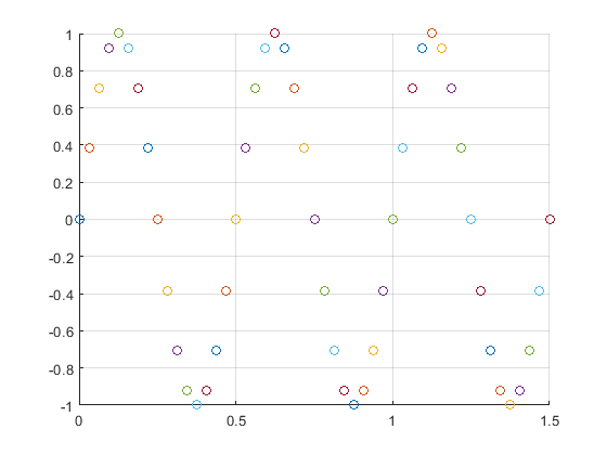
3.5.1: Create a 2D x-y Sine-Wave Plot with a for Loop

By Carey A. Smith

2-Dimensional plots of a time sequence can be easily created in MATLAB and in Octave.

Octave needs a graphics toolkit to plot graph. Insert this line in your code before creating your first figure:

graphics_toolkit("qt") % Do not use with MATLAB

If that doen't work, try this version:
graphics_toolkit("fltk")

The graphics toolkit is only for Octave. It is not needed for MATLAB and will cause an error if attempted.

For more information on graphics toolkit options, see:

https://docs.octave.org/interpreter/Graphics-Toolkits.html
 

The key lines of code for creating a plot in both MATLAB and Octave are:

• figure; % Open a figure window. The plot is created in this figure window.
• plot(t, sin_t, 'o')
  • The first variable, t, is the x coordinate of the point.
  • The second variable, sin_t, is the y coordinate of the point.
  • The 'o' means to use a circle for point's marker.
• hold on; % Let additional points be plotted on the same figure

It can be useful to code this example together as a class.

Example \(\PageIndex{1}\) Plot points of a sine wave

% Compute and plot points of a sine wave
% using a script with a "for loop"
clear all; % Clear all variables
clc; % Clear the console (computer screen)
close all; % close all figures
format compact; % Don't insert blank lines on the console

graphics_toolkit("fltk") % Include this line when using Octave. Not for Matlab.

%% Initialize variables
period = 0.5; % seconds
t_end = 3*period; % The end of the interval
dt = period/16; % time between points

%%
figure; % Open a figure window
xlim([0,t_end]) % Set the x-axis to be 0 to t_end
ylim([-1,1]) % Set the x-axis to be -1 to 1
grid on; % Draw grid lines
hold on; % Let additional points be plotted on the same figure
%%
for t = 0 : dt : t_end % t = 0, dt, 2*dt, ... t_end
    % Compute the sine for the current value of t
    sin_t = sin(2*pi*t/period);
    plot(t, sin_t, 'o')
    pause(0.3) % pause long enuf to see each point as it is plotted
end

Solution