3.7.1: Series Additional Material

By Carey A. Smith

There are 2 methods to sum a series. Let the variable "term" be computed value of the current value and the variable "total" be the running sum.

Method 1: Use a temporary variable, "total_new", to make it clear what is happening:

total_new = total + term;  % Add the previous total and the current term to get the new total.

total = total_new;  % Reset total to the new value

Method 2: Directly assign the new value of "total" to be equal to current value of total + term:

total = total + term;  % Replace the previous total with the sum of the current term + term

These 2 methods are equivalent. The first method is more obvious what is happening. The second is method common among experienced programmers. It may be slightly faster.

Note: Variable names other than "total"--such as "series_sum--are often used in codes. 

Warning: Do not using "sum" as a variable, because that would be a name collision with the built-in function sum().

.

Example \(\PageIndex{1}\) Power Series1

% Clear any variables etc.
clear all; close all; format compact; clc;
% Initialize these variables:
n = 6;    % The number of terms in the series
A0 = 4; % The first value
r = 1/2;  % The ratio of successive terms
% Write a for loop that computes the terms in the series which are computed with this expression:
%   A(k) = A0*r^k;

%% Method 1:
total = 0;  % Initialize the total
for k = 1:n
  A(k) = A0*r^k;
  total_new = total + A(k);
  total = total_new;
end
A % This displays all the values of the vector A
disp(['Method 1 total = ',num2str(total)])

%% Method 2:
total = 0;  % Initialize the total
for k = 1:n
  A(k) = A0*r^k;
  total = total + A(k);
end
A % This displays all the values of the vector A
disp(['Method 2 total = ',num2str(total)])

Solution

Add example text here.

.

Exercise \(\PageIndex{1}\) atan(x) Taylor's series and absolute error

The Taylor's series for the arctangent function is:

atan(x) = x - x³/3 + x⁵/5 - x⁷/7 + ...

The general formula for the k^th term is computed with these 2 lines of code:

m = (2*k-1) % This generates 1, 3, 5, 7, ...

term = (-1)^(k-1)*x^m / m   % (-1)^(k-1) = 1, -1, 1, -1, ...

Because the sign changes from term to term, this is called an alternating series.

(1 pt) Write a Matlab m-file script. This script will have a "for loop". The details of the for loop are described below.

(1 pt) Put these lines of code at the beginning of your file:

% Compute the Taylor's series for atan(x)
% Clear any variables; close any figures; eliminate white space; clear the console
clear all; close all; format compact; clc;
% Open a figure for plotting the partial sums

% Octave needs graphics toolkit to plot graph.
graphics_toolkit("fltk") % Do not use with MATLAB
figure;
hold on;
grid on;

(1 pt) Initialize these variables:

x = pi/5 % Set the x-value
atan_series = 0; % Initialize the series' sum

(2 pts) Write a for loop. Let k = the for-loop index. k goes from 1 to 8

(3 pts) Inside the for loop, compute term as specified above for each iteration.

Then add term to the previous value of atan_series with this code (method 1):

atan_series_new = atan_series + term

atan_series = atan_series_new

(1 pt) Inside the for loop, also plot the kth partial sum with this code:

plot(k, atan_series,'o');

(1 pt) After the for loop, display the sum and the last term with these lines of code:

atan_series % Display the series sum

term % Display the last term that was calculated

(1 pt) Compute and display atan_Matlab = atan(x) [Matlab's buit-in function]

(1 pt) Compute and display the absolute error = abs( atan_series - atan_Matlab)

If the code is done correctly, the absolute error should be < 0.001

Answer

Add texts here. Do not delete this text first

.

Example \(\PageIndex{1}\) Bessel Function

The image of a star thru a space telescope, which has no aberrations, is called an Airy pattern, shown in this image:

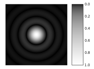
Figure \(\PageIndex{1}\): Airy pattern

(Airy pattern image [en.Wikipedia.org], This work has been released into the public domain by its author, Sakurambo at English Wikipedia.)

The formula for a cross-section of the Airy pattern intensity is:

\[ I(\theta) = I_0 \left[ \frac{2J_1(k*a*sin\theta)}{k*a*sin\theta} \right]^2 = I_0 \left[ \frac{2J_1(x)}{x} \right]^2 \]

where J₁(x) is the 1^st-order Bessel function of the 1^st kind.

This Bessel function is approximated by this infinite series with α = 1:

\[J_\alpha (x) = \sum_{m=0}^\infty \frac{(-1)^m}{m!*\Gamma(m+\alpha+1)} * \left(\frac{x}{2}\right)^{(2m+\alpha)} \]

For m!, use the Matlab function factorial(m)

Г(p) = the Gamma function. In Matlab this function is gamma(p).

When is a positive integer, gamma(p) = (p-1)!

Instructions:

1. Set x = 0.5
2. Write a for loop to sum the terms of this Bessel function series, J_α(x), for m = 0 to 10.
3. Display the last term
4. Display the resulting sum

Solution

term = 1.5697e-27
J1_x = 0.24227

..