10.3: Fourier Transforms

By Carey A. Smith

The code in this section is in file: FFT_demo_1.m

FFT_demo_1.m

The Fourier Transform is defined as the integral of a signal multiplied by sine and cosine functions of frequencies which are multiples of a fundamental frequency.

A common use of FFT's is to find the frequency components of a signal.

% Computers compute the Fourier Transform of a signal vector using an algorithm called the "Fast Fourier Transform" or FFT.

MATLAB's function is fft(). The input is a vector y of signal values sampled at times specified by a vector t. For a signal vector, y, and a time vector, t, the syntax to properly scale the frequencies is:

y_FFT = (sqrt(t(end)))*fft(y);

Example \(\PageIndex{1}\) Spectral Analysis 1

%% This example shows the use of the Fourier Transform for spectral analysis.

clear all; close all; format compact; format short; clc;

% Create a time vector

nt = 256; % Vector length (A power of 2 is most efficient)

dt = 0.01; % (sec) Sampling interval

t = (0:1:(nt-1))*dt; % (sec) Time vector

%% Create a Signal vector

bias = 0; % Average value

f1 = 4.0 % (Hz) 1st frequency

a1 = 4.0 % Magnitude of the 1st frequency

f2 = 10.0 % (Hz) 2nd frequency

a2 = 2.0 % Magnitude of the 2nd frequency

y = bias + a1*sin(2*pi*f1*t) + a2*sin(2*pi*f2*t);

y_power = mean(y.^2) % power in the signal

%% Plot y vs. t

figure;

plot(t,y)

title('Original Signal vs. Time')

xlabel('Time (s)')

grid on;

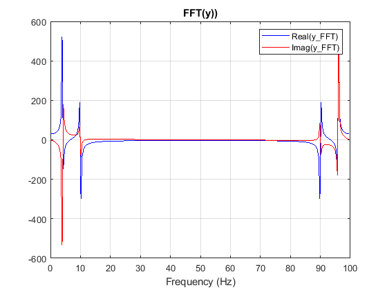
%% Compute the Fourier Transform

y_FFT = (sqrt(t(end)))*fft(y); % Scale the FFT

f_max = (1/dt) % (Hz) Maximum frequency = Sample frequency

df = (1/dt)/nt % (Hz) Freq. interval

freqs = (0:1:(nt-1))*df; % Frequencies of the FFT

%% Plot the FFT of y

% The FFT result vector has complex values

figure;

plot(freqs,real(y_FFT),'b');

hold on;

plot(freqs,imag(y_FFT),'r');

legend('Real(y\_FFT)','Imag(y\_FFT)');

title('FFT(y))');

xlabel('Frequency (Hz)');

grid on;

%% Convert the complex Fourier Transform to magnitude squared.

y_FFT2 = (df/nt^2)*(y_FFT.*conj(y_FFT)); % (df/nt^2)is a scaled factor

y_FFT2_power = sum(y_FFT2)

% 10.02

figure;

plot(freqs,y_FFT2);

title('FFT2 Power)');

xlabel('Frequency (Hz)');

grid on;

%% The Nyquist–Shannon sampling theorem says

% you can only measure frequencies up to 1/2 the sampling frequency.

f_Nyquist = f_max/2

% You can see that the power plot is symmetric about the center frequency.

% The frequencies > f_Nyquist are equivalent to negative frequncies.

% We double the lower frequncies (except for 0 Hz)

% and delete the high frequencies.

y_FFT3 = [y_FFT2(1), 2*y_FFT2(2:(nt/2)), y_FFT2(nt/2+1)];

y_FFT3_power = sum(y_FFT3)

% 10.02

freqs3 = freqs(1:(nt/2+1));

figure;

plot(freqs3,y_FFT3);

title('y\_FFT3 Power Spectrum');

xlabel('Frequency (Hz)');

grid on;

Figure \(\PageIndex{1}\): Signal vs. time

Figure \(\PageIndex{1}\): The FFT's real and imaginary components

Figure \(\PageIndex{1}\): Power Spectrum, 0 to 100 Hz

Figure \(\PageIndex{1}\): Power Spectrum, folder onto 0 to 50 Hz

.

Exercise \(\PageIndex{1}\) Spectral Analysis 2

Modify the code in the above example as follows.

Change the 2 frequencies to 6 Hz and 16 Hz.

Call this signal y0. (This is without noise)

Use randn() to add a noise vector to y0 with a mean of 0 and a standard deviation of 4. 

y  = y0 + 4*randn(size(y));

This adds noise of all frequencies. Such noise is called “white noise”.

The Power Spectrum should be strong at the 2 main frequencies. A small amount of random power should be at all the other frequencies.

Answer

Add texts here. Do not delete this text first.

Exercise \(\PageIndex{2}\) Spectral Analysis with large noise

Using your code from the previous exercise (Spectral Analysis 2), increase the noise to a point where the noise makes it somewhat hard to see the periodic part of signal in the plot of y vs. t.

Describe what the Fourier Transform plot shows.

Are the frequencies of the 2 sine waves identifiable?

Answer

Add texts here. Do not delete this text first.