1.1.3: Local Position Tracking - Odometry

Dead reckoning, which tracks location by integrating a moving system's speed and heading over time, forms the backbone of many mobile robot navigation systems. The simplest form of dead

Figure 1.1: A mobile robot with pose \((x, y, \theta)\).

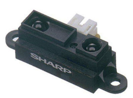
(a) The Sharp IR distance sensor

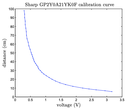
(b) Calibration curve

Figure 1.2: Sharp GP2Y0A21YK0F infrared distance sensor and its calibration curve.

reckoning for land-based vehicles is odometry, which derives speed and heading information from sensed wheel rotations.

Figure 1.3: A quadrature rotary encoder and its output for clockwise and counterclockwise rotation.

\(d_{\text {wheel }}\)	\(2.71\)	inches
\(L_{\text {baseline }}\)	\(5.25\)	inches
\(N\)	\(60\)	ticks

Table 1.1: Mobile robot parameters.

By "summing up" the increments, we can compute the total cumulative distances \(s_{\text {left }}\) and \(s_{\text {right }}\) traveled by the left and right wheels, respectively.

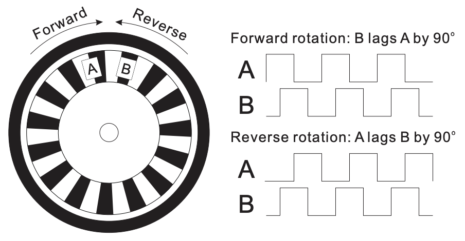
The variables time, LeftTicks, and RightTicks from assignment1. mat contain sample times \(t^{k}\) (in seconds) and cumulative left and right encoder counts \(n_{\text {left }}\) and \(n_{\text {right }}\), respectively, recorded during a single test run of a mobile robot. Note that the quadrature decoding for forward and reverse rotation has already been incorporated in the data, such that cumulative counts increase for forward rotation and decrease for reverse rotation. The values of the odometry constants for the mobile robot are given in Table \(1 .\)

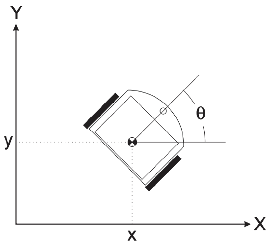
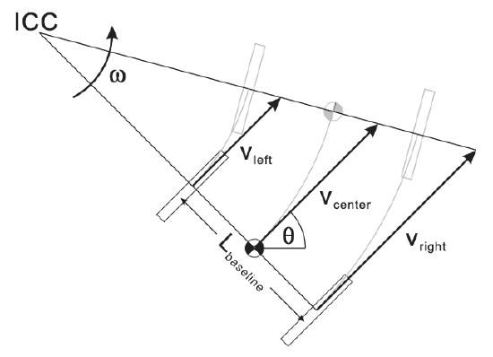
For a mobile robot with two-wheel differential drive, in which the two (left and right) driven wheels can be controlled independently, the linear velocities \(v_{\text {left }}\) and \(v_{\text {right }}\) at the two wheels must (assuming no slippage of the wheels) be both directed in (or opposite to) the direction \(\theta\) of the robot’s current heading. The motion of the robot can thus be completely described by the velocity \(v_{\text {center }}\) of a point lying midway between the two wheels and the angular velocity \(\omega\) about an instantaneous center of curvature (ICC) lying somewhere in line with the two wheels, as shown in Figure 1.4.

Figure 1.4: Robot trajectory.

and \(L_{\rm baseline}\) is the distance between the points of contact of the two wheels. We can then integrate these velocities to track the pose \([x(t), y(t), \theta(t)]\) of the robot over time as \[\begin{aligned} &x(t)=\int_{0}^{t} v_{\text {center }}(t) \cos [\theta(t)] d t, \\ &y(t)=\int_{0}^{t} v_{\text {center }}(t) \sin [\theta(t)] d t, \\ &\theta(t)=\int_{0}^{t} \omega(t) d t . \end{aligned}\] In terms of the sample times \(t^{k}\), we can write these equations as \[\begin{aligned} x^{k} &=x^{k-1}+\int_{t^{k-1}}^{t^{k}} v_{\text {center }}(t) \cos [\theta(t)] d t, \\ y^{k} &=y^{k-1}+\int_{t^{k-1}}^{t^{k}} v_{\text {center }}(t) \sin [\theta(t)] d t, \\ \theta^{k} &=\theta^{k-1}+\int_{t^{k-1}}^{t^{k}} \omega(t) d t . \end{aligned}\]