2.2.2: Discrete Bivariate Random Variables (Random Vectors)

Joint Distributions

So far, we have consider scalar random variables, each of whose outcomes is described by a single value. In this section, we extend the concept to random variables whose outcome are vectors. For simplicity, we consider a random vector of the form \[(X, Y) \text {, }\] where \(X\) and \(Y\) take on \(J_{X}\) and \(J_{Y}\) values, respectively. Thus, the random vector \((X, Y)\) takes on \(J=J_{X} \cdot J_{Y}\) values. The probability mass function associated with \((X, Y)\) is denoted by \(f_{X, Y}\). Similar to the scalar case, the probability mass function assigns a probability to each of the possible outcomes, i.e. \[f_{X, Y}\left(x_{i}, y_{j}\right)=p_{i j}, \quad i=1, \ldots, J_{X}, \quad j=1, \ldots, J_{Y} .\] Again, the function must satisfy \[\begin{aligned} 0 \leq p_{i j} \leq 1, \quad i=1, \ldots, J_{X}, \quad j=1, \ldots, J_{Y}, \\ \sum_{j=1}^{J_{Y}} \sum_{i=1}^{J_{X}} p_{i j} &=1 . \end{aligned}\] Before we introduce key concepts that did not exist for a scalar random variable, let us give a simple example of joint probability distribution.

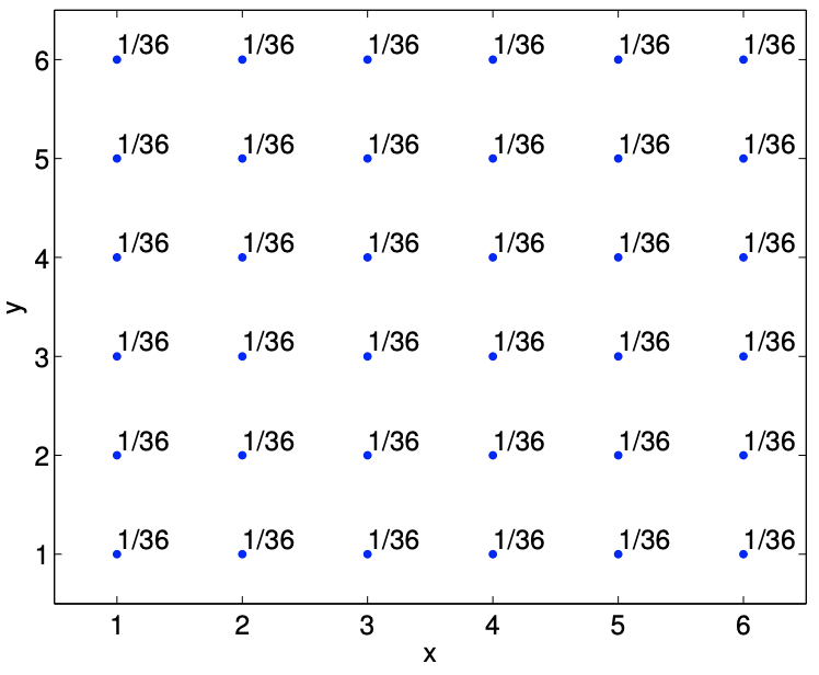
Example 9.2.1 rolling two dice

As the first example, let us consider rolling two dice. The first die takes on \(x_{i}=i, i=1, \ldots, 6\), and the second die takes on \(y_{j}=j, j=1, \ldots, 6\). The random vector associated with rolling the two dice is \[(X, Y),\] where \(X\) takes on \(J_{X}=6\) values and \(Y\) takes on \(J_{Y}=6\) values. Thus, the random vector \((X, Y)\) takes on \(J=J_{X} \cdot J_{Y}=36\) values. Because (for a fair die) each of the 36 outcomes is equally likely, the probability mass function \(f_{X, Y}\) is \[f_{X, Y}\left(x_{i}, y_{j}\right)=\frac{1}{36}, \quad i=1, \ldots, 6, \quad j=1, \ldots, 6 .\] The probability mass function is shown graphically in Figure \(\underline{9.4}\).

Figure 9.4: The probability mass function for rolling two dice.

Characterization of Joint Distributions

Now let us introduce a few additional concepts useful for describing joint distributions. Throughout this section, we consider a random vector \((X, Y)\) with the associated probability distribution \(f_{X, Y}\). First is the marginal density, which is defined as \[f_{X}\left(x_{i}\right)=\sum_{j=1}^{J_{Y}} f_{X, Y}\left(x_{i}, y_{j}\right), \quad i=1, \ldots, J_{X}\] In words, marginal density of \(X\) is the probability distribution of \(X\) disregarding \(Y\). That is, we ignore the outcome of \(Y\), and ask ourselves the question: How frequently does \(X\) take on the value \(x_{i}\) ? Clearly, this is equal to summing the joint probability \(f_{X, Y}\left(x_{i}, j_{j}\right)\) for all values of \(y_{j}\). Similarly, the marginal density for \(Y\) is \[f_{Y}\left(y_{j}\right)=\sum_{i=1}^{J_{X}} f_{X, Y}\left(x_{i}, y_{j}\right), \quad j=1, \ldots, J_{Y}\] Again, in this case, we ignore the outcome of \(X\) and ask: How frequently does \(Y\) take on the value \(y_{j}\) ? Note that the marginal densities are valid probability distributions because \[f_{X}\left(x_{i}\right)=\sum_{j=1}^{J_{Y}} f_{X, Y}\left(x_{i}, y_{j}\right) \leq \sum_{k=1}^{J_{X}} \sum_{j=1}^{J_{Y}} f_{X, Y}\left(x_{k}, y_{j}\right)=1, \quad i=1, \ldots, J_{X}\] and \[\sum_{i=1}^{J_{X}} f_{X}\left(x_{i}\right)=\sum_{i=1}^{J_{X}} \sum_{j=1}^{J_{Y}} f_{X, Y}\left(x_{i}, y_{j}\right)=1\] The second concept is the conditional probability, which is the probability that \(X\) takes on the value \(x_{i}\) given \(Y\) has taken on the value \(y_{j}\). The conditional probability is denoted by \[f_{X \mid Y}\left(x_{i} \mid y_{j}\right), \quad i=1, \ldots, J_{X}, \quad \text { for a given } y_{j}\] The conditional probability can be expressed as \[f_{X \mid Y}\left(x_{i} \mid y_{j}\right)=\frac{f_{X, Y}\left(x_{i}, y_{j}\right)}{f_{Y}\left(y_{j}\right)} .\] In words, the probability that \(X\) takes on \(x_{i}\) given that \(Y\) has taken on \(y_{j}\) is equal to the probability that both events take on \(\left(x_{i}, y_{j}\right)\) normalized by the probability that \(Y\) takes on \(y_{j}\) disregarding \(x_{i}\). We can consider a different interpretation of the relationship by rearranging the equation as \[f_{X, Y}\left(x_{i}, y_{j}\right)=f_{X \mid Y}\left(x_{i} \mid y_{j}\right) f_{Y}\left(y_{j}\right)\] and then summing on \(j\) to yield \[f_{X}\left(x_{i}\right)=\sum_{j=1}^{J_{Y}} f\left(x_{i}, y_{j}\right)=\sum_{j=1}^{J_{Y}} f_{X \mid Y}\left(x_{i} \mid y_{j}\right) f_{Y}\left(y_{j}\right) .\] In other words, the marginal probability of \(X\) taking on \(x_{i}\) is equal to the sum of the probabilities of \(X\) taking on \(x_{i}\) given \(Y\) has taken on \(y_{j}\) multiplied by the probability of \(Y\) taking on \(y_{j}\) disregarding \(x_{i}\).

From (9.2), we can derive Bayes’ law (or Bayes’ theorem), a useful rule that relates conditional probabilities of two events. First, we exchange the roles of \(x\) and \(y\) in \(\underline{(9.2)}\), obtaining \[f_{Y, X}\left(y_{j}, x_{i}\right)=f_{Y \mid X}\left(y_{j} \mid x_{i}\right) f_{X}\left(x_{i}\right) .\] But, since \(f_{Y, X}\left(y_{j}, x_{i}\right)=f_{X, Y}\left(x_{i}, y_{j}\right)\), \[f_{Y \mid X}\left(y_{j} \mid x_{i}\right) f_{X}\left(x_{i}\right)=f_{X \mid Y}\left(x_{i} \mid y_{j}\right) f_{Y}\left(y_{j}\right),\] and rearranging the equation yields \[f_{Y \mid X}\left(y_{j} \mid x_{i}\right)=\frac{f_{X \mid Y}\left(x_{i} \mid y_{j}\right) f_{Y}\left(y_{j}\right)}{f_{X}\left(x_{i}\right)} .\] Equation (9.3) is called Bayes’ law. The rule has many useful applications in which we might know one conditional density and we wish to infer the other conditional density. (We also note the theorem is fundamental to Bayesian statistics and, for example, is exploited in estimation and inverse problems - problems of inferring the underlying parameters of a system from measurements.)

Example 9.2.2 marginal and conditional density of rolling two dice

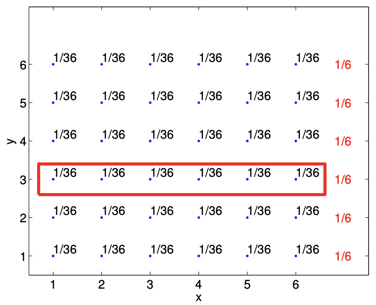
Let us revisit the example of rolling two dice, and illustrate how the marginal density and conditional density are computed. We recall that the probability mass function for the problem is \[f_{X, Y}(x, y)=\frac{1}{36}, \quad x=1, \ldots, 6, y=1, \ldots, 6 .\] The calculation of the marginal density of \(X\) is illustrated in Figure 9.5(a). For each \(x_{i}\), \(i=1, \ldots, 6\), we have \[f_{X}\left(x_{i}\right)=\sum_{j=1}^{6} f_{X, Y}\left(x_{i}, y_{j}\right)=\frac{1}{36}+\frac{1}{36}+\frac{1}{36}+\frac{1}{36}+\frac{1}{36}+\frac{1}{36}=\frac{1}{6}, \quad i=1, \ldots, 6 .\] We can also deduce this from intuition and arrive at the same conclusion. Recall that marginal density of \(X\) is the probability density of \(X\) ignoring the outcome of \(Y\). For this two-dice rolling

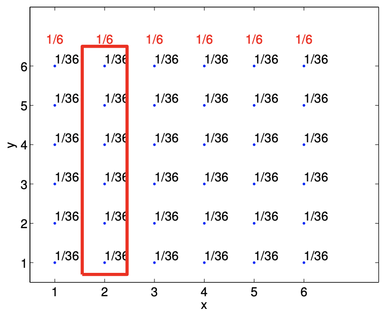
(a) marginal density, \(f_{X}\)

(b) marginal density, \(f_{Y}\)

Figure 9.5: Illustration of calculating marginal density \(f_{X}(x=2)\) and \(f_{Y}(y=3)\).

example, it simply corresponds to the probability distribution of rolling a single die, which is clearly equal to \[f_{X}(x)=\frac{1}{6}, \quad x=1, \ldots, 6 .\] Similar calculation of the marginal density of \(Y, f_{Y}\), is illustrated in Figure \(9.5(\mathrm{~b})\). In this case, ignoring the first die \((X)\), the second die produces \(y_{j}=j, j=1, \ldots, 6\), with the equal probability of \(1 / 6\).

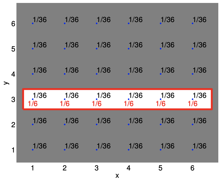
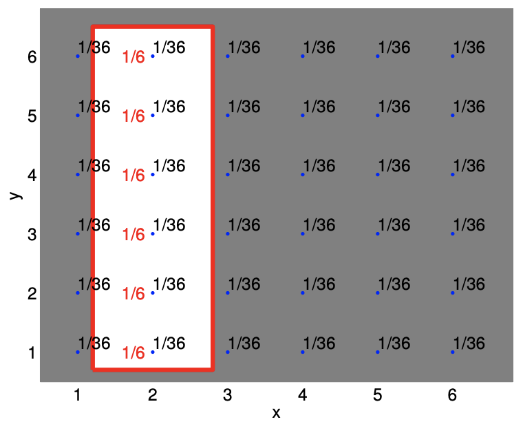
Let us now illustrate the calculation of conditional probability. As the first example, let us compute the conditional probability of \(X\) given \(Y\). In particular, say we are given \(y=3\). As shown in Figure 9.6(a), the joint probability of all outcomes except those corresponding to \(y=3\) are irrelevant (shaded region). Within the region with \(y=3\), we have six possible outcomes, each with the equal probability. Thus, we have \[f_{X \mid Y}(x \mid y=3)=\frac{1}{6}, \quad x=1, \ldots, 6\] Note that, we can compute this by simply considering the select set of joint probabilities \(f_{X, Y}(x, y=\) 3) and re-normalizing the probabilities by their sum. In other words, \[f_{X \mid Y}(x \mid y=3)=\frac{f_{X, Y}(x, y=3)}{\sum_{i=1}^{6} f_{X, Y}\left(x_{i}, y=3\right)}=\frac{f_{X, Y}(x, y=3)}{f_{Y}(y=3)}\] which is precisely equal to the formula we have introduced earlier.

Similarly, Figure \(9.6(\mathrm{~b})\) illustrates the calculation of the conditional probability \(f_{Y \mid X}(y, x=2)\). In this case, we only consider joint probability distribution of \(f_{X, Y}(x=2, y)\) and re-normalize the density by \(f_{X}(x=2)\).

(a) conditional density, \(f_{X \mid Y}(x \mid y=3)\)

(b) conditional density, \(f_{Y \mid X}(y \mid x=2)\)

Figure 9.6: Illustration of calculating conditional density \(f_{X \mid Y}(x \mid y=3)\) and \(f_{Y \mid X}(y \mid x=2)\).

The fact that the probability density is simply a product of marginal densities means that we can draw \(X\) and \(Y\) separately according to their respective marginal probability and then form the random vector \((X, Y)\).

Using conditional probability, we can connect our intuitive understanding of independence with the precise definition. Namely, \[f_{X \mid Y}\left(x_{i} \mid y_{j}\right)=\frac{f_{X, Y}\left(x_{i}, y_{j}\right)}{f_{Y}\left(y_{j}\right)}=\frac{f_{X}\left(x_{i}\right) f_{Y}\left(y_{j}\right)}{f_{Y}\left(y_{j}\right)}=f_{X}\left(x_{i}\right)\] That is, the conditional probability of \(X\) given \(Y\) is no different from the probability that \(X\) takes on \(x\) disregarding \(y\). In other words, knowing the outcome of \(Y\) adds no additional information about the outcome of \(X\). This agrees with our intuitive sense of independence.

We have discussed the notion of "or" and related it to the union of two sets. Let us now briefly discuss the notion of "and" in the context of joint probability. First, note that \(f_{X, Y}(x, y)\) is the probability that \(X=x\) and \(Y=y\), i.e. \(f_{X, Y}(x, y)=P(X=x\) and \(Y=y)\). More generally, consider two events \(A\) and \(B\), and in particular \(A\) and \(B\), which is the intersection of \(A\) and \(B\), \(A \cap B\). If the two events are independent, then \[P(A \text { and } B)=P(A) P(B)\] and hence \(f_{X, Y}(x, y)=f_{X}(x) f_{Y}(y)\) which we can think of as probability of \(P(A \cap B)\). Pictorially, we can associate event \(A\) with \(X\) taking on a specified value as marked in Figure \(9.5(\) a \()\) and event \(B\) with \(Y\) taking on a specified value as marked in Figure 9.5(b). The intersection of \(A\) and \(B\) is the intersection of the two marked regions, and the joint probability \(f_{X, Y}\) is the probability associated with this intersection.

To solidify the idea of independence, let us consider two canonical examples involving coin flips.

Example 9.2.3 independent events: two random variables associated with two independent coin flips

Let us consider flipping two fair coins. We associate the outcome of flipping the first and second coins with random variables \(X\) and \(Y\), respectively. Furthermore, we associate the values of 1 and

Figure 9.7: The probability mass function for flipping two independent coins.

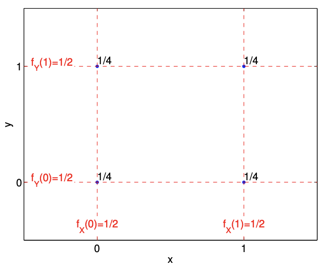
0 to head and tail, respectively. We can associate the two flips with a random vector \((X, Y)\), whose possible outcomes are \[(0,0), \quad(0,1), \quad(1,0), \quad \text { and }(1,1)\] Intuitively, the two variables \(X\) and \(Y\) will be independent if the outcome of the second flip, described by \(Y\), is not influenced by the outcome of the first flip, described by \(X\), and vice versa.

We postulate that it is equally likely to obtain any of the four outcomes, such that the joint probability mass function is given by \[f_{X, Y}(x, y)=\frac{1}{4}, \quad(x, y) \in\{(0,0),(0,1),(1,0),(1,1)\}\] We now show that this assumption implies independence, as we would intuitively expect. In particular, the marginal probability density of \(X\) is \[f_{X}(x)=\frac{1}{2}, \quad x \in\{0,1\}\] since \((\) say \() P(X=0)=P((X, Y)=(0,0))+P((X, Y)=(0,1))=1 / 2\). Similarly, the marginal probability density of \(Y\) is \[f_{Y}(y)=\frac{1}{2}, \quad y \in\{0,1\}\] We now note that \[f_{X, Y}(x, y)=f_{X}(x) \cdot f_{Y}(y)=\frac{1}{4}, \quad(x, y) \in\{(0,0),(0,1),(1,0),(1,1)\}\] which is the definition of independence.

The probability mass function of \((X, Y)\) and the marginal density of \(X\) and \(Y\) are shown in Figure 9.7. The figure clearly shows that the joint density of \((X, Y)\) is the product of the marginal density of \(X\) and \(Y\). Let us show that this agrees with our intuition, in particular by considering the probability of \((X, Y)=(0,0)\). First, the relative frequency that \(X\) takes on 0 is \(1 / 2\). Second, of the events in which \(X=0,1 / 2\) of these take on \(Y=0\). Note that this probability is independent of the value that \(X\) takes. Thus, the relative frequency of \(X\) taking on 0 and \(Y\) taking on 0 is \(1 / 2\) of \(1 / 2\), which is equal to \(1 / 4\).

Figure 9.8: The probability mass function for flipping two independent coins.

We can also consider conditional probability of an event that \(X\) takes on 1 given that \(Y\) takes on 0 . The conditional probability is \[f_{X \mid Y}(x=1 \mid y=0)=\frac{f_{X, Y}(x=1, y=0)}{f_{Y}(y=0)}=\frac{1 / 4}{1 / 2}=\frac{1}{2} .\] This probability is equal to the marginal probability of \(f_{X}(x=1)\). This agrees with our intuition; given that two events are independent, we gain no additional information about the outcome of \(X\) from knowing the outcome of \(Y\).

Example 9.2.4 non-independent events: two random variables associated with a single

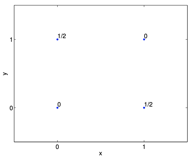
Let us now consider flipping a single coin. We associate a Bernoulli random variables \(X\) and \(Y\) with \[X=\left\{\begin{array}{ll} 1, & \text { head } \\ 0, & \text { tail } \end{array} \quad \text { and } Y=\left\{\begin{array}{ll} 1, & \text { tail } \\ 0, & \text { head } \end{array} .\right.\right.\] Note that a head results in \((X, Y)=(1,0)\), whereas a tail results in \((X, Y)=(0,1)\). Intuitively, the random variables are not independent, because the outcome of \(X\) completely determines \(Y\), i.e. \(X+Y=1\).

Let us show that these two variables are not independent. We are equally like to get a head, \((1,0)\), or a tail, \((0,1)\). We cannot produce \((0,0)\), because the coin cannot be head and tail at the same time. Similarly, \((1,1)\) has probably of zero. Thus, the joint probability density function is \[f_{X, Y}(x, y)= \begin{cases}\frac{1}{2}, & (x, y)=(0,1) \\ \frac{1}{2}, & (x, y)=(1,0) \\ 0, & (x, y)=(0,0) \text { or }(x, y)=(1,1) .\end{cases}\] The probability mass function is illustrated in Figure \(\underline{9.8}\).

The marginal density of each of the event is the same as before, i.e. \(X\) is equally likely to take on 0 or 1 , and \(Y\) is equally like to take on 0 or 1. Thus, we have \[\begin{aligned} &f_{X}(x)=\frac{1}{2}, \quad x \in\{0,1\} \\ &f_{Y}(y)=\frac{1}{2}, \quad y \in\{0,1\} . \end{aligned}\] For \((x, y)=(0,0)\), we have \[f_{X, Y}(x, y)=0 \neq \frac{1}{4}=f_{X}(x) \cdot f_{Y}(y) .\] So, \(X\) and \(Y\) are not independent.

We can also consider conditional probabilities. The conditional probability of \(x=1\) given that \(y=0\) is \[f_{X \mid Y}(x=1 \mid y=0)=\frac{f_{X, Y}(x=1, y=0)}{f_{Y}(y=0)}=\frac{1 / 2}{1 / 2}=1 .\] In words, given that we know \(Y\) takes on 0, we know that \(X\) takes on 1. On the other hand, the conditional probability of \(x=1\) given that \(y=1\) is \[f_{X \mid Y}(x=0 \mid y=0)=\frac{f_{X, Y}(x=0, y=0)}{f_{Y}(y=0)}=\frac{0}{1 / 2}=0 .\] In words, given that \(Y\) takes on 1 , there is no way that \(X\) takes on 1 . Unlike the previous example that associated \((X, Y)\) with two independent coin flips, we know with certainty the outcome of \(X\) given the outcome of \(Y\), and vice versa.

We have seen that independence is one way of describing the relationship between two events. Independence is a binary idea; either two events are independent or not independent. Another concept that describes how closely two events are related is correlation, which is a normalized covariance. The covariance of two random variables \(X\) and \(Y\) is denoted by \(\operatorname{Cov}(X, Y)\) and defined as \[\operatorname{Cov}(X, Y) \equiv E\left[\left(X-\mu_{X}\right)\left(Y-\mu_{Y}\right)\right] .\] The correlation of \(X\) and \(Y\) is denoted by \(\rho_{X Y}\) and is defined as \[\rho_{X Y}=\frac{\operatorname{Cov}(X, Y)}{\sigma_{X} \sigma_{Y}},\] where we recall that \(\sigma_{X}\) and \(\sigma_{Y}\) are the standard deviation of \(X\) and \(Y\), respectively. The correlation indicates how strongly two random events are related and takes on a value between \(-1\) and 1 . In particular, two perfectly correlated events take on 1 (or \(-1\) ), and two independent events take on 0 .

Two independent events have zero correlation because \[\begin{aligned} \operatorname{Cov}(X, Y) &=E\left[\left(X-\mu_{X}\right)\left(Y-\mu_{Y}\right)\right]=\sum_{j=1}^{J_{Y}} \sum_{i=1}^{J_{X}}\left(x_{i}-\mu_{X}\right)\left(y_{j}-\mu_{Y}\right) f_{X, Y}\left(x_{i}, y_{j}\right) \\ &=\sum_{j=1}^{J_{Y}} \sum_{i=1}^{J_{X}}\left(x_{i}-\mu_{X}\right)\left(y_{j}-\mu_{Y}\right) f_{X}\left(x_{i}\right) f_{Y}\left(y_{j}\right) \\ &=\left[\sum_{j=1}^{J_{Y}}\left(y_{j}-\mu_{Y}\right) f_{Y}\left(y_{j}\right)\right] \cdot\left[\sum_{i=1}^{J_{X}}\left(x_{i}-\mu_{X}\right) f_{X}\left(x_{i}\right)\right] \\ &=E\left[Y-\mu_{Y}\right] \cdot E\left[X-\mu_{X}\right]=0 \cdot 0=0 . \end{aligned}\] The third inequality follows from the definition of independence, \(f_{X, Y}\left(x_{i}, y_{j}\right)=f_{X}\left(x_{i}\right) f_{Y}\left(y_{j}\right)\). Thus, if random variables are independent, then they are uncorrelated. However, the converse is not true in general.