5.3: Continuity Equation

In this chapter and the next three chapters, the conservation equations will be applied to the control volume. In this chapter, the mass conservation will be discussed. The system mass change is

\[ \dfrac{D\,m_{sys}}{Dt} = \dfrac{D}{Dt} \int_{V_{sys}} \rho dV = 0
\label{mass:eq:Dmdt}

\]

The system mass after some time, according Figure 5.1, is made of

\[ m_{sys} = m_{c.v.} + m_a - m_{c}
\label{mass:eq:mSysAfter}

\]

The change of the system mass is by definition is zero. The change with time (time derivative of equation (??) results in

\[ 0 = \dfrac{D\,m_{sys}}{Dt} = \dfrac{d\,m_{c.v.}}{dt} + \dfrac{d\, m_a}{dt} - \dfrac{d\,m_{c}}{dt}
\label{mass:eq:mSysAfterdt}
\]

The first term in equation (??) is the derivative of the mass in the control volume and at any given time is

\[ \label{mass:eq:masst}
\dfrac{d\,m_{c.v.} (t)}{dt} = \dfrac{d}{dt} \int_{V_{c.v.}}\rho\,dV
\] and is a function of the time.

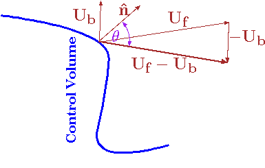
Fig. 5.3 Schematics of velocities at the interface.

The interface of the control volume can move. The actual velocity of the fluid leaving the control volume is the relative velocity (see Figure 5.3). The relative velocity is

\[ \overrightarrow{U_r} = \overrightarrow{U_f} - \overrightarrow{U_{b}}
\label{mass:eq:relativeU}
\]

Where \(U_f\) is the liquid velocity and \(U_b\) is the boundary velocity (see Figure 5.3). The velocity component that is perpendicular to the surface is

\[ \label{mass:eq:reltiveA}
U_{rn} = -\hat{n}\cdot \overrightarrow{U_r} = U_r \, \cos \theta
\] Where \(\hat{n}\) is an unit vector perpendicular to the surface. The convention of direction is taken positive if flow out the control volume and negative if the flow is into the control volume. The mass flow out of the control volume is the system mass that is not included in the control volume. Thus, the flow out is

\[ \label{mass:eq:madta}
\dfrac{d\, m_a}{dt} = \int_{S_{cv}} \rho_s \,U_{rn} dA
\] It has to be emphasized that the density is taken at the surface thus the subscript \(s\). In the same manner, the flow rate in is

\[ \label{mass:eq:madtb}
\dfrac{d\, m_b}{dt} = \int_{S_{c.v.}} \rho_s\,U_{rn} dA
\] It can be noticed that the two equations (??) and (??) are similar and can be combined, taking the positive or negative value of \(U_{rn}\) with integration of the entire system as

\[ \label{mass:eq:mdtCombine}
\dfrac{d\, m_a}{dt} - \dfrac{d\, m_b}{dt} = \int_{S_{cv}} \rho_s\,U_{rn} \, dA
\] applying negative value to keep the convention. Substituting equation (??) into equation (??) results in

Continuity

\[ \label{mass:eq:intS}
\dfrac{d}{dt} \int_{c.v.} \rho_s dV =
-\int_{S_{cv}} \rho\,U_{rn} \, dA
\]

Equation (??) is essentially accounting of the mass. Again notice the negative sign in surface integral. The negative sign is because flow out marked positive which reduces of the mass (negative derivative) in the control volume. The change of mass change inside the control volume is net flow in or out of the control system.

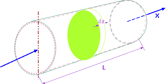
Fig. 5.4 Schematics of flow in in pipe with varying density as a function time for example 5.1.}

The next example is provided to illustrate this concept.

Example 5.1

The density changes in a pipe, due to temperature variation and other reasons, can be approximated as

\[ \nonumber
\dfrac{\rho(x,t)}{\rho_0} = \left( 1 - \dfrac{x}{L\dfrac{}{}}\right)^2 \cos {\dfrac{t}{t_0}}.
\]

The conduit shown in Figure 5.4 length is \(L\) and its area is \(A\). Express the mass flow in and/or out, and the mass in the conduit as function of time. Write the expression for the mass change in the pipe.

Solution 5.1

Here it is very convenient to choose a non-deformable control volume that is inside the conduit \(dV\) is chosen as \(\pi\,R^2\,dx\). Using equation (??), the flow out (or in) is
\begin{align*}
\dfrac{d}{dt} \int_{c.v.} \rho dV =
\dfrac{d}{dt} \int_{c.v.}
\overbrace{\rho_0 \left(1 - \dfrac{x}{L} \right)^2 \cos\left( \dfrac{t}{t_0} \right)} ^{\rho(t)}
\overbrace{\pi\,R^2\, dx}^{dV}
\end{align*}
The density is not a function of radius, \(r\) and angle, \(\theta\) and they can be taken out the integral as
\begin{align*}
\dfrac{d}{dt} \int_{c.v.} \rho dV =
\pi\,R^2 \dfrac{d}{dt} \int_{c.v.}\rho_0 \left(1-\dfrac{x}{L\dfrac{}{}} \right)^2 \cos \left(
\dfrac{t}{t_0 \dfrac{}{}}\right) dx
\end{align*}
which results in
\begin{align*}
\text{Flow Out} = \overbrace{ \pi\,R^2}^{A}
\dfrac{d}{dt} \int_{0}^{L} \rho_0 \left(1-\dfrac{x}{L \dfrac{}{}}\right)^2 \cos {\dfrac{t}{t_0}} dx =
- \dfrac{\pi\,R^2\,L\, \rho_0}{3\,t_0} \, \sin\left( \dfrac{t}{t_0} \right)
\end{align*}
The flow out is a function of length, \(L\), and time, \(t\), and is the change of the mass in the control volume.

Contributors and Attributions

• Dr. Genick Bar-Meir. Permission is granted to copy, distribute and/or modify this document under the terms of the GNU Free Documentation License, Version 1.2 or later or Potto license.