
1.3: Algebra of Complex Numbers
- Page ID
- 9949

\( \newcommand{\vecs}[1]{\overset { \scriptstyle \rightharpoonup} {\mathbf{#1}} } \)
\( \newcommand{\vecd}[1]{\overset{-\!-\!\rightharpoonup}{\vphantom{a}\smash {#1}}} \)
\( \newcommand{\dsum}{\displaystyle\sum\limits} \)
\( \newcommand{\dint}{\displaystyle\int\limits} \)
\( \newcommand{\dlim}{\displaystyle\lim\limits} \)
\( \newcommand{\id}{\mathrm{id}}\) \( \newcommand{\Span}{\mathrm{span}}\)
( \newcommand{\kernel}{\mathrm{null}\,}\) \( \newcommand{\range}{\mathrm{range}\,}\)
\( \newcommand{\RealPart}{\mathrm{Re}}\) \( \newcommand{\ImaginaryPart}{\mathrm{Im}}\)
\( \newcommand{\Argument}{\mathrm{Arg}}\) \( \newcommand{\norm}[1]{\| #1 \|}\)
\( \newcommand{\inner}[2]{\langle #1, #2 \rangle}\)
\( \newcommand{\Span}{\mathrm{span}}\)
\( \newcommand{\id}{\mathrm{id}}\)
\( \newcommand{\Span}{\mathrm{span}}\)
\( \newcommand{\kernel}{\mathrm{null}\,}\)
\( \newcommand{\range}{\mathrm{range}\,}\)
\( \newcommand{\RealPart}{\mathrm{Re}}\)
\( \newcommand{\ImaginaryPart}{\mathrm{Im}}\)
\( \newcommand{\Argument}{\mathrm{Arg}}\)
\( \newcommand{\norm}[1]{\| #1 \|}\)
\( \newcommand{\inner}[2]{\langle #1, #2 \rangle}\)
\( \newcommand{\Span}{\mathrm{span}}\) \( \newcommand{\AA}{\unicode[.8,0]{x212B}}\)
\( \newcommand{\vectorA}[1]{\vec{#1}} % arrow\)
\( \newcommand{\vectorAt}[1]{\vec{\text{#1}}} % arrow\)
\( \newcommand{\vectorB}[1]{\overset { \scriptstyle \rightharpoonup} {\mathbf{#1}} } \)
\( \newcommand{\vectorC}[1]{\textbf{#1}} \)
\( \newcommand{\vectorD}[1]{\overrightarrow{#1}} \)
\( \newcommand{\vectorDt}[1]{\overrightarrow{\text{#1}}} \)
\( \newcommand{\vectE}[1]{\overset{-\!-\!\rightharpoonup}{\vphantom{a}\smash{\mathbf {#1}}}} \)
\( \newcommand{\vecs}[1]{\overset { \scriptstyle \rightharpoonup} {\mathbf{#1}} } \)
\(\newcommand{\longvect}{\overrightarrow}\)
\( \newcommand{\vecd}[1]{\overset{-\!-\!\rightharpoonup}{\vphantom{a}\smash {#1}}} \)
\(\newcommand{\avec}{\mathbf a}\) \(\newcommand{\bvec}{\mathbf b}\) \(\newcommand{\cvec}{\mathbf c}\) \(\newcommand{\dvec}{\mathbf d}\) \(\newcommand{\dtil}{\widetilde{\mathbf d}}\) \(\newcommand{\evec}{\mathbf e}\) \(\newcommand{\fvec}{\mathbf f}\) \(\newcommand{\nvec}{\mathbf n}\) \(\newcommand{\pvec}{\mathbf p}\) \(\newcommand{\qvec}{\mathbf q}\) \(\newcommand{\svec}{\mathbf s}\) \(\newcommand{\tvec}{\mathbf t}\) \(\newcommand{\uvec}{\mathbf u}\) \(\newcommand{\vvec}{\mathbf v}\) \(\newcommand{\wvec}{\mathbf w}\) \(\newcommand{\xvec}{\mathbf x}\) \(\newcommand{\yvec}{\mathbf y}\) \(\newcommand{\zvec}{\mathbf z}\) \(\newcommand{\rvec}{\mathbf r}\) \(\newcommand{\mvec}{\mathbf m}\) \(\newcommand{\zerovec}{\mathbf 0}\) \(\newcommand{\onevec}{\mathbf 1}\) \(\newcommand{\real}{\mathbb R}\) \(\newcommand{\twovec}[2]{\left[\begin{array}{r}#1 \\ #2 \end{array}\right]}\) \(\newcommand{\ctwovec}[2]{\left[\begin{array}{c}#1 \\ #2 \end{array}\right]}\) \(\newcommand{\threevec}[3]{\left[\begin{array}{r}#1 \\ #2 \\ #3 \end{array}\right]}\) \(\newcommand{\cthreevec}[3]{\left[\begin{array}{c}#1 \\ #2 \\ #3 \end{array}\right]}\) \(\newcommand{\fourvec}[4]{\left[\begin{array}{r}#1 \\ #2 \\ #3 \\ #4 \end{array}\right]}\) \(\newcommand{\cfourvec}[4]{\left[\begin{array}{c}#1 \\ #2 \\ #3 \\ #4 \end{array}\right]}\) \(\newcommand{\fivevec}[5]{\left[\begin{array}{r}#1 \\ #2 \\ #3 \\ #4 \\ #5 \\ \end{array}\right]}\) \(\newcommand{\cfivevec}[5]{\left[\begin{array}{c}#1 \\ #2 \\ #3 \\ #4 \\ #5 \\ \end{array}\right]}\) \(\newcommand{\mattwo}[4]{\left[\begin{array}{rr}#1 \amp #2 \\ #3 \amp #4 \\ \end{array}\right]}\) \(\newcommand{\laspan}[1]{\text{Span}\{#1\}}\) \(\newcommand{\bcal}{\cal B}\) \(\newcommand{\ccal}{\cal C}\) \(\newcommand{\scal}{\cal S}\) \(\newcommand{\wcal}{\cal W}\) \(\newcommand{\ecal}{\cal E}\) \(\newcommand{\coords}[2]{\left\{#1\right\}_{#2}}\) \(\newcommand{\gray}[1]{\color{gray}{#1}}\) \(\newcommand{\lgray}[1]{\color{lightgray}{#1}}\) \(\newcommand{\rank}{\operatorname{rank}}\) \(\newcommand{\row}{\text{Row}}\) \(\newcommand{\col}{\text{Col}}\) \(\renewcommand{\row}{\text{Row}}\) \(\newcommand{\nul}{\text{Nul}}\) \(\newcommand{\var}{\text{Var}}\) \(\newcommand{\corr}{\text{corr}}\) \(\newcommand{\len}[1]{\left|#1\right|}\) \(\newcommand{\bbar}{\overline{\bvec}}\) \(\newcommand{\bhat}{\widehat{\bvec}}\) \(\newcommand{\bperp}{\bvec^\perp}\) \(\newcommand{\xhat}{\widehat{\xvec}}\) \(\newcommand{\vhat}{\widehat{\vvec}}\) \(\newcommand{\uhat}{\widehat{\uvec}}\) \(\newcommand{\what}{\widehat{\wvec}}\) \(\newcommand{\Sighat}{\widehat{\Sigma}}\) \(\newcommand{\lt}{<}\) \(\newcommand{\gt}{>}\) \(\newcommand{\amp}{&}\) \(\definecolor{fillinmathshade}{gray}{0.9}\)The complex numbers form a mathematical “field” on which the usual operations of addition and multiplication are defined. Each of these operations has a simple geometric interpretation.
Addition and Multiplication
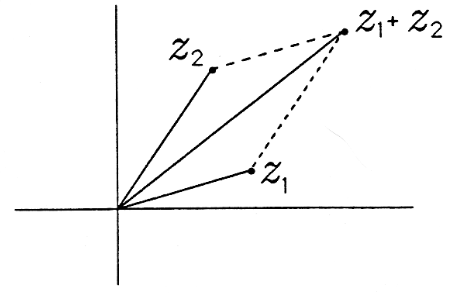
The complex numbers \(z_1\) and \(z_2\) are added according to the rule
\[z_1+z_2 = (x_1+jy_1) + (x_2+jy_2) = (x_1+x_2) + j(y_1+y_2) \nonumber \]
We say that the real parts add and the imaginary parts add. As illustrated in the Figure, the complex number \(z_1+z_2\) is computed from a “parallelogram rule,” wherein \(z_1+z_2\) lies on the node of a parallelogram formed from \(z_1\) and \(z_2\).
Let \(z_1 = r_1e^{jθ_1}\) and \(z_2 = r_2e^{jθ_2}\). Find a polar formula \(z_3 = r_3e^{jθ_3}\) for \(z_3 = z_1 + z_2\) that involves only the variables \(r_1,r_2,θ_1,\) and \(θ_2\). The formula for \(r_3\) is the “law of cosines.”
The product of \(z_1\) and \(z_2\) is
\[z_1z_2=(x_1+jy_1)(x_2+jy_2) = (x_1x_2−y_1y_2)+j(y_1x_2+x_1y_2) \nonumber \]
If the polar representations for \(z_1\) and \(z_2\) are used, then the product may be written as 1
\[\begin{align}
z_{1} z_{2} &=\quad r_{1} e^{j \theta_{1}} r_{2} e^{j \theta_{2}} \label{} \\
&=\left(r_{1} \cos \theta_{1}+j r_{1} \sin \theta_{1}\right)\left(r_{2} \cos \theta_{2}+j r_{2} \sin \theta_{2}\right) \label{}\\
&=\left(r_{1} \cos \theta_{1} r_{2} \cos \theta_{2}-r_{1} \sin \theta_{1} r_{2} \sin \theta_{2}\right) \label{}\\
&+j\left(r_{1} \sin \theta_{1} r_{2} \cos \theta_{2}+r_{1} \cos \theta_{1} r_{2} \sin \theta_{2}\right) \label{}\\
&=\quad r_{1} r_{2} \cos \left(\theta_{1}+\theta_{2}\right)+j r_{1} r_{2} \sin \left(\theta_{1}+\theta_{2}\right) \label{}\\
&=\quad r_{1} r_{2} e^{j\left(\theta_{1}+\theta_{2}\right)} \label{}
\end{align} \nonumber \]
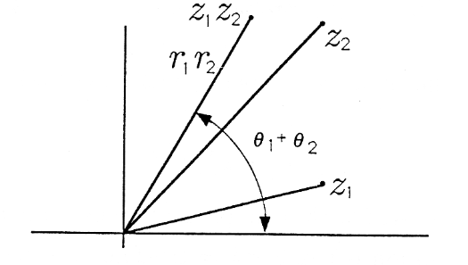
We say that the magnitudes multiply and the angles add. As illustrated in Figure, the product \(z_1z_2\) lies at the angle \((θ_1+θ_2)\)
Rotation
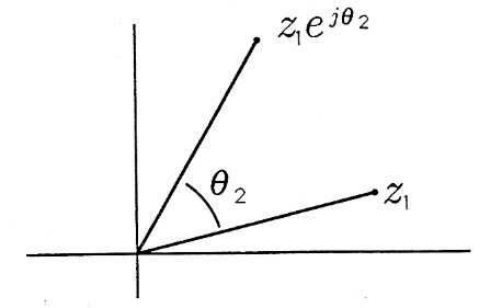
There is a special case of complex multiplication that will become very important in our study of phasors in the chapter on Phasors. When \(z_1\) is the complex number \(z_1=r_1e^{jθ_1}\) and \(z_2\) is the complex number \(z_2=r_1e^{jθ_2}\), then the product of \(z_1\) and \(z_2\) is
\[z_1z_2=z_1e^{jθ_2}=r_1e^{j(θ_1+θ_2)} \nonumber \]
As illustrated in Figure, \(\)z_1z_2\) is just a rotation of \(z_1\) through the angle \(θ_2\)
Begin with the complex number \(z_1=x+jy=re^{jθ}\). Compute the complex number \(z_2=jz_1\) in its Cartesian and polar forms. The complex number \(z_2\) is sometimes called perp\((z_1)\). Explain why by writing perp\((z_1)\) as \(z_1e^{jθ_2}\). What is \(θ_2\)? Repeat this problem for \(z_3=−jz_1\).
Powers
If the complex number \(z_1\) multiplies itself \(N\) times, then the result is
\[(z_1)^N=r^N_1e^{jNθ_1} \nonumber \]
This result may be proved with a simple induction argument. Assume \(zk_1=rk_1e^{jkθ_1}\). (The assumption is true for \(k=1\).) Then use the recursion \(z^{k+1}_1=z^k_1z_1=r^{k+1}_1e^{j(k+1)θ_1}\). Iterate this recursion (or induction) until \(k+1=N\). Can you see that, as \(n\) ranges from \(n=1,...,N,\) the angle of z§ranges from \(θ_1\) to \(2θ_1\),..., to \(Nθ_1\) and the radius ranges from \(r_1\) to \(r^2_1\),..., to \(r^N_1\) ? This result is explored more fully in Problem 1.19
Complex Conjugate
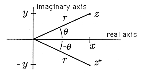
Corresponding to every complex number \(z= x+jy=re^{jθ}\) is the complex conjugate
\[z^∗=x−jy=re^{−jθ} \nonumber \]
The complex number \(z\) and its complex conjugate are illustrated in the Figure. The recipe for finding complex conjugates is to “change \(j\) to \(−j\). This changes the sign of the imaginary part of the complex number.
Magnitude Squared
The product of \(z\) and its complex conjugate is called the magnitude squared of \(z\) and is denoted by \(|z|^2\)
\[|z|^2=z^∗z=(x−jy)(x+jy)=x^2+y^2=re^{−jθ}re^{jθ}=r^2 \nonumber \]
Note that \(|z|=r\) is the radius, or magnitude, that we defined in "Geometry of Complex Numbers".
Write \(z^∗\) as \(z^∗=zw\). Find \(w\) in its Cartesian and polar forms.
Prove that angle \((z_2z^∗_1)=θ_2−θ_1\).
Show that the real and imaginary parts of \(z=x+jy\) may be written as
\[\mathrm{Re}[z]=\frac 1 2 (z+z^∗) \nonumber \]
\[\mathrm{Im}[z]=\overline{2j}(z−z^∗) \nonumber \]
Commutativity, Associativity, and Distributivity
The complex numbers commute, associate, and distribute under addition and multiplication as follows:
\[z_1+z_2 = z_2+z_1 \nonumber \]
\[z_1z_2 = z_2z_1 \nonumber \]
\[(z_1+z_2)+z_3=z_1+(z_2+z_3) \nonumber \]
\[z_1(z_2z_3)=(z_1z_2)z_3 \nonumber \]
\[z_1(z_2+z_3)=z_1z_2+z_1z_3 \nonumber \]
Identities and Inverses
In the field of complex numbers, the complex number \(0+j0\) (denoted by 0) plays the role of an additive identity, and the complex number \(1+j0\) (denoted by 1) plays the role of a multiplicative identity:
\[z+0=z=0+z \nonumber \]
\[z1=z=1z \nonumber \]
In this field, the complex number \(−z=−x+j(−y)\) is the additive inverse of \(z\), and the complex number \(z^{−1} = \frac {x} {x^2+y^2} + j \left(/frac {−y} {x^2+y^2} \right) is the multiplicative inverse:
\[z+(−z) = 0 \nonumber \]
\[zz^{−1} = 1 \nonumber \]
Show that the additive inverse of \(z=re^{jθ}\) may be written as \(re^{j(θ+π)}\).
Show that the multiplicative inverse of \(z\) may be written as
\[z^{−1} = \frac {1} {z^∗z} z^∗ = \frac {1} {x^2 + y^2} (x−jy) \nonumber \]
Show that \(z^∗z\) is real. Show that \(z^{−1}\) may also be written as
\[z^{−1} = r^{−1}e^{−jθ} \nonumber \]
Plot \(z\) and \(z^{−1}\) for a representative \(z\).
Prove \((j)^{−1} = −j\).
Find \(z^{−1}\) when \(z = 1+j1\)
Prove \((z^{−1})^∗ = (z^∗)^{−1} = r^{−1}e^{jθ} = \frac {1} {z^∗z} z\). Plot \(z\) and \((z^{−1})^∗\) for a representative \(z\).
Find all of the complex numbers \(z\) with the property that \(jz = −z^∗\). Illustrate these complex numbers on the complex plane
Demo 1.2 (MATLAB)
Create and run the following script file (name it Complex Numbers) 2
clear, clg

j=sqrt(-1)

z1=1+j*.5,z2=2+j*1.5

z3=z1+z2,z4=z1*z2

z5=conj(z1),z6=j*z2

avis([-4 4 -4 4]),axis('square'),plot(z1,'0')

hold on

plot(z2,'0'),plot(z3,'+'),plot(z4,'*'),

plot(z2,'0'),plot(z3,'+'),plot(z4,'*'),

plot(z5,'x'),plot(z6,'x')

With the help of Appendix 1, you should be able to annotate each line of this program. View your graphics display to verify the rules for add, multiply, conjugate, and perp. See Figure.
Prove that \(z^0 = 1\).
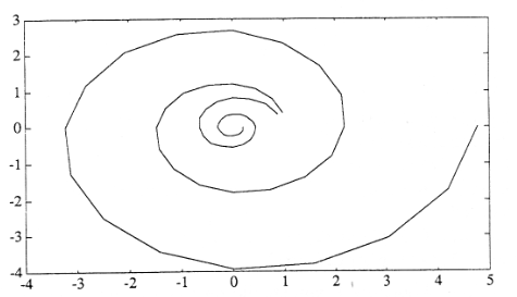
(MATLAB) Choose \(z_1 = 1.05e^{j2π/16}\) and \(z_2 = 0.95e^{j2π/16}\). Write a MATLAB program to compute and plot \(z^n_1\) and \(z^n_2\) for \(n = 1,2,...,32\). You should observe a figure like the one below.
Footnotes
- We have used the trigonometric identities \(cos(θ_1+θ_2) = cos{θ_1}cos{θ_2} − sin{θ_1}sin{θ_2}\) and \(sin(θ_1+θ_2) = sin{θ_1}cos{θ_2} + cos{θ_1}sin{θ_2}\) to derive this result.
- If you are using PC-MATLAB, you will need to name your file cmplxnos.m