5.1: Introduction to Vector Graphics

Acknowledgements

Fundamentals of Interactive Computer Graphics by J. D. Foley and A. Van Dam, ©1982 Addison-Wesley Publishing Company, Inc., Reading, Massachusetts, was used extensively as a reference book during development of this chapter. Star locations were obtained from the share- ware program “Deep Space” by David Chandler, who obtained them from the “Skymap” database of the National Space Science Data Center.

Notes to Teachers and Students:

In this chapter we introduce matrix data structures that may be used to represent two- and three-dimensional images. The demonstration program shows students how to create a function file for creating images from these data structures. We then show how to use matrix transformations for translating, scaling, and rotating images. Projections are used to project three-dimensional images onto two-dimensional planes placed at arbitrary locations. It is precisely such projections that we use to get perspective drawings on a two-dimensional surface of three-dimensional objects. The numerical experiment encourages students to manipulate a star field and view it from several points in space.

Once again we consider certain problems essential to the chapter development. For this chapter be sure not to miss the following exercises: Exercise 2 in "Two-Dimensional Image Transformations", Exercise 1 in "Homogeneous Coordinates", Exercise 2 in "Homogeneous Coordinates", Exercise 5 in "Three-Dimensional Homogeneous Coordinates", and Exercise 2 in "Projections".

Introduction

Pictures play a vital role in human communication, in robotic manufacturing, and in digital imaging. In a typical application of digital imaging, a CCD camera records a digital picture frame that is read into the memory of a digital computer. The digital computer then manipulates this frame (or array) of data in order to crop, enlarge or reduce, enhance or smooth, translator rotate the original picture. These procedures are called digital picture processing or computer graphics. When a sequence of picture frames is processed and displayed at video frame rates (30 frames per second), then we have an animated picture.

In this chapter we use the linear algebra we developed in The chapter on Linear Algebra to develop a rudimentary set of tools for doing computer graphics on line drawings. We begin with an example: the rotation of a single point in the \((x,y)\) plane.

Example \(\PageIndex{1}\)

Point \(P\) has coordinates (3,1) in the \((x,y)\) plane as shown in Figure 1. Find the coordinates of the point \(P'\), which is rotated \(\frac{\pi}{6}\) radians from \(P\).

Figure \(\PageIndex{1}\): Rotating a Single Point in the \((x,y)\) Plane

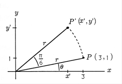
To solve this problem, we can begin by converting the point \(P\) from rectangular coordinates to polar coordinates. We have

\[r=\sqrt{x^{2}+y^{2}}=\sqrt{10} \nonumber \]

\[\theta=\tan ^{-1}\left(\frac{y}{x}\right) \approx 0.3217 \nonumber \] radian.

The rotated point \(P'\) has the same radius \(r\), and its angle is \(\theta + \frac{\pi}{6}\). We now convert back to rectangular coordinates to find \(x'\) and \(y'\) for point \(P'\):

\[x^{\prime}=r \cos \left(\theta+\frac{\pi}{6}\right) \approx \sqrt{10} \cos (0.8453) \approx 2.10 \nonumber \]

\[y^{\prime}=r \sin \left(\theta+\frac{\pi}{6}\right) \approx \sqrt{10} \sin (0.8453) \approx 2.37 \text { . } \nonumber \]

So the rotated point \(P'\) has coordinates (2.10, 2.37).

Now imagine trying to rotate the graphical image of some complex object like an airplane. You could try to rotate all 10,000 (or so) points in the same way as the single point was just rotated. However, a much easier way to rotate all the points together is provided by linear algebra. In fact, with a single linear algebraic operation we can rotate and scale an entire object and project it from three dimensions to two for display on a flat screen or sheet of paper.

In this chapter we study vector graphics, a linear algebraic method of storing and manipulating computer images. Vector graphics is especially suited to moving, rotating, and scaling (enlarging and reducing) images and objects within images. Cropping is often necessary too, although it is a little more difficult with vector graphics. Vector graphics also allows us to store objects in three dimensions and then view the objects from various locations in space by using projections.

In vector graphics, pictures are drawn from straight lines.¹ A curve can be approximated as closely as desired by a series of short, straight lines. Clearly some pictures are better suited to representation by straight lines than are others. For example, we can achieve a fairly good representation of a building or an airplane in vector graphics, while a photograph of a forest would be extremely difficult to convert to straight lines. Many computer-aided design (CAD) programs use vector graphics to manipulate mechanical drawings.

When the time comes to actually display a vector graphics image, it may be necessary to alter the representation to match the display device. Personal computer display screens are divided into thousands of tiny rectangles called picture elements, or pixels. Each pixel is either off (black) or on (perhaps with variable intensity and/or color). With a CRT display, the electron beam scans the rows of pixels in a raster pattern. To draw a line on a pixel display device, we must first convert the line into a list of pixels to be illuminated. Dot matrix and laser printers are also pixel display devices, while pen plotters and a few specialized CRT devices can display vector graphics directly. We will let MATLAB do the conversion to pixels and automatically handle cropping when necessary.

We begin our study of vector graphics by representing each point in an image by a vector. These vectors are arranged side-by-side into a matrix \(G\) containing all the points in the image. Other matrices will be used as operators to perform the desired transformations on the image points. For example, we will find a matrix \(R\), which functions as a rotation: the matrix product \(RG\) represents a rotated version of the original image \(G\).

Footnotes

1. It is possible to extend these techniques to deal with some types of curves, but we will consider only straight lines for the sake of simplicity.