7.1: Aggregate Data Types

The number of ways in which pieces of data can be arranged is far greater than the number of different atomic types. These various ways all have names, some of them nerdy and/or exotic like “hash tables,” “binary search trees,” and “skip lists.” Nevertheless, there are again three basic ones which will form the basis of our study: they’re called arrays, associative arrays, and tables. As before, we’ll consider each one conceptually first, and then look at how to use them in Python.

Arrays

An array is simply a sequence of items, all in a row. We call those items the “elements” of the array. So an array could have ten whole numbers as its elements, or a thousand strings of text, or a million real numbers.

Normally, we will deal with homogeneous arrays, in which all the elements are of the same type; this turns out to be what you want 99% of the time. Some languages (including Python) do permit creating a heterogeneous array, which could hold (say) three whole numbers, sixteen reals, and four strings of text all mixed together. But usually you’re using an array to contain a bunch of related values, like the current balances of all the accounts in your bank, or the Twitter screen names of all a user’s followees.

Figure 7.1.1 shows what those two examples would look like conceptually. One has four strings of text, and the other five real numbers. Note that each entire set of elements is one variable. We might call the left one “followees” and the right one “balances.”

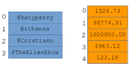
Figure \(\PageIndex{1}\): Two arrays.

Worthy of special note are the numbers on the left-hand side. These numbers are called the indices (singular: index) of the array. They exist simply so we have a way to talk about the individual elements. I could say “element #2 of the followees array” to refer to @Cristiano.

And yes, you noticed that the index numbers start with 0, not 1. Yes, this is weird. The reason I did that it is because nearly all programming languages (including Python) number their array elements starting with zero, so you might as well just start getting used to it now. It’s really not hard once you get past the initial weirdness.

Arrays are the most basic kind of aggregate data there is, and they are the workhorse of a whole lot of Data Science processing. Sometimes they’re called lists, vectors, or sequences, by the way. (When a particular concept has lots of different names, you know it’s important.)

Associative Arrays

An associative array, by contrast, has no index numbers. And its elements are slightly more complicated: instead of just bare values, an associative array contains key-value pairs. Figure 7.1.2 shows a couple of examples. The left-hand side of each picture shows the keys, and the right-hand side the corresponding value.

With an associative array, you don’t ask “what’s element #3?” like you do with a regular array. Instead, you ask “what value is associated with the "Baltimore" key?” And out pops your answer ("Ravens").

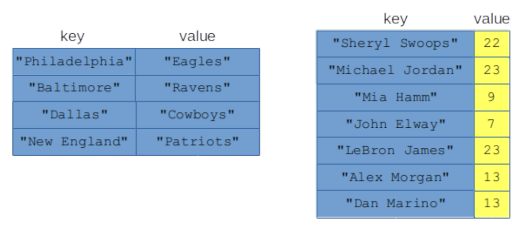
Figure \(\PageIndex{2}\): Two associative arrays.

All access to the associative array is through the keys: you can change the value that goes with a key, retrieve the value that goes with a key, or even retrieve and process all the keys and their associated values sequentially.1 In that third case, the order in which you’ll receive the key-value pairs is undefined (which means “not guaranteed to be consistent” or “not necessarily what you’d expect.”) This underscores the fact that there isn’t any reliable “first” key-value pair, or second, or last. They’re just kind of all equally “in there.” Your mental model of an associative array should just think of keys that are mapped to values (we say that "Dallas" is “mapped” to "Cowboys") without any implied order. (Sure, the "Philadelphia"/"Eagles" pair is at the top of the picture, but that’s only because I had to put something at the top of the picture, and I chose Philadelphia at random. It doesn’t have any meaningful primacy though.)

Note a couple things about Figure 7.1.2. First, the keys in an associative array will almost always (and for us, always) be homogeneous. Similarly, the values will be homogeneous. But the keys might not be of the same type as the values. In the left picture, both keys and values are text, but in the right picture, the keys are text and the values (uniform numbers of famous athletes) are whole numbers. This is perfectly healthy and good.

Second, realize that the keys in an associative array must be unique – this means that there can be no duplicate keys. If we tried to create a second "Alex Morgan" (oh, if only...) with a different value, that new value would replace Alex’s current value, not sit alongside the first one as an additional key-value pair.

The reverse is not true, however: the values of an associative array may very well not be unique. In the left-hand picture they are, but in the right-hand picture there are duplicates: both Jordan and LeBron wore #23 in their stellar careers, while Hall of Famer quarterback Dan Marino once chose the same uniform number that Alex wears today. This isn’t a problem, because we always access the information in an associative array through the keys. Asking “what number did Mia Hamm wear?” gives us a well-defined answer. Asking “which famous athlete wore #23?” does not. That’s why we can’t ask that second question (and aren’t meant to).

Tables

Lastly, we have the table, which in Data Science is positively ubiquitous. In Figure 7.1.3 we return to the pinterest.com example, with a table of their most popular users. As you can see, it has more going on that than the previous two aggregate data types. Still, it’s pretty straightforward to wrap your head around.

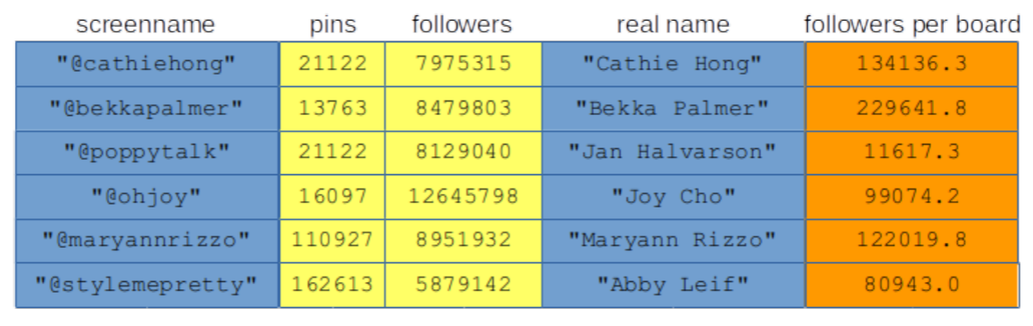
Figure \(\PageIndex{3}\): A table

Unlike the other two aggregate data types, tables are full-on twodimensional. There’s (theoretically) no limit to how many rows and how many columns they can have. By the way, it’s important to get those two terms straight: rows go across, and columns go up and down. (Think of the columns in the Trinkle Rotunda.) Also, the typical table has many, many more rows than columns, so they’re super tall and skinny, not short and fat.

Although the rows of a table are often heterogeneous, each column must be homogeneous. You can see that with a glance at Figure 7.3. Each column represents a specific type of data – in this case, some statistic or piece of information about a Pinterest user. Clearly all screen names should be of a text type, all “number of pins or followers” should be whole numbers, etc. It doesn’t make sense otherwise.

As with the other types, the whole dog-gone table – no matter how many millions of rows it might have – is one variable with a single name. Also, just like with associative arrays, there normally isn’t any implied order to the rows. Many implementations of these data types (including Python/Pandas) will actually let you specify “the first row” or “the 53^rd row,” but that always makes me cringe because conceptually, there isn’t any such thing. They’re just “rows” that are all “in there.”

“Querying” Tables (and other things)

Now you might be wondering how to actually “get at” the individual values of a table. Unlike arrays, there’s no index number. And unlike associative arrays, there’s no key. How then to address, say, the @poppytalk row?

The answer will turn out to be something called a query, which is a geeky way of saying “a set of criteria which will match some, but not all, of the rows and/or columns.” For instance, we might say “tell me the pin count for @ohjoy.” Or, “give me all the information for any user who has more than 100,000 followers per board and at least 20,000 pins.” Those specific requirements will restrict the table to a subset of its rows and/or columns. We’ll learn the syntax for that later. It’s a bit tricky but very powerful.

By the way, it turns out we’ll actually be using the concept of a query for arrays and associative arrays as well. So strictly speaking, a query isn’t just a “table thing.” However, they’re especially invaluable for tables, since they’re essentially the only way to access individual elements.