8.2: The NumPy 'ndarray'

The actual data type that the NumPy package provides is called an ndarray, which stands for “n-dimensional array.” If that sounds heady, it kind of is, although in this course we’re only ever going to use a one-dimensional array, which is super simple to understand. In fact, it looks exactly like the examples in Figure 7.1.1.

“One-dimensional” just means that there is a single index number, and the elements are all in a line.²

Creating ndarrays

There are many different ways to create an ndarray. We’ll learn four of them.

Way 1: np.array([])

The first is to use the array() function of the NumPy package, and give it all the values explicitly. Here’s the code to reproduce the Figure 7.1.1 examples:

Code \(\PageIndex{1}\) (Python):

followees = np.array(['@katyperry','@rihanna','@TheEllenShow'])

balances = np.array([1526.73, 98774.91, 1000000, 4963.12, 123.19])

It’s simple, but don’t miss the syntactical gotcha: you must include a pair of boxies inside the bananas. Why? Reasons.³ For now, just memorize that for this function – and this function only – we use “([...stuff...])” instead of “(...stuff...)” when we call it.

By the way, the attentive reader might object to me calling array() a function, instead of a method. Isn’t there a word-and-a-dot before it, and isn’t that a “method thing?” Shrewd of you to think that, but actually no, and the reason is that “np” isn’t the name of a variable, but the name of a package. When we say “np.array()” what we’re saying is: “Python, please call the array() function from the np package.” The word-and-dot syntax does double-duty.

We can call the type() function, as we did back on p. 17, to verify that yes indeed we have created ndarrays:

Code \(\PageIndex{2}\) (Python):

print(type(followees))

print(type(balances))

| numpy.ndarray

| numpy.ndarray

This is useful, but sometimes we want to know what underlying atomic data type the array is comprised of. To do that, we attach “.dtype” (confusingly, without bananas this time) to the end of the variable name. “.dtype” stands for “data type.” Here goes:

Code \(\PageIndex{3}\) (Python):

print(followees.dtype)

print(balances.dtype)

|dtype('<U13')

| dtype('float64')

Whoa, what does that stuff mean? It’s a bit hard on the eyes, but let me explain. The underlying data type of followees is (bizarrely) "U13" which in English means “strings of Unicode characters⁴ , each of which is 13 characters long or less.” (If you bother to count, you’ll discover that the longest string in our followees array is the last one, ’@TheEllenShow’, which is exactly 13 characters long.) The “float64” thing means “floats, each of which is represented with 64 bits⁵ in memory.

You don’t need to worry about any of those details. All you need to know is: if an array’s dtype has "<U" in it, then it’s composed of strings; and if it has the word “int” or “float” in it, it means one of those two old friends from chapter 3.

Incidentally, you’ll recall from chapter 7 that an array is homogeneous, which means all its elements are of the same type. NumPy enforces this. If you try to combine them:

Code \(\PageIndex{4}\) (Python):

weird = np.array([3, 4.9, 8])

strange = np.array([18, 73.0, 'bob', 22.8])

you’ll discover that NumPy converts them to all be of the same type:

Code \(\PageIndex{5}\) (Python):

print(weird)

print(weird.dtype)

print(strange)

print(strange.dtype)

|[ 3. 4.9 8. ]

| dtype('<U3')

| ['18' '73.0' 'bob' '22.8']

| dtype('float64')

See how the ints 3 and 8 from the first array were converted into the floats 3. and 8.; meanwhile, all of the numerical elements of the second array got converted to strs. (If you think about it, that’s the only direction the conversions could go.)

Way 2: np.zeros()

It will often be useful to create an array, possibly a large one, with all elements equal to zero initially. Among other scenarios, we often need to use a bunch of counter variables to, well, count things. (Recall our incrementing technique from Section 5.1) Suppose, for example, that we had a giant array that held the numbers of likes that each Instagram photo had. When someone likes a photo, that photo’s appropriate element in the array should be incremented (raised in value) by one. Similarly, if someone unlikes it, then its value in the array should be decremented by one.

An easy way to do this is NumPy’s zeros() function:

Code \(\PageIndex{1}\) (Python):

photo_likes = np.zeros(40000000000)

(although I’ll bet you don’t have enough memory on your laptop to actually store an array this size! Instagram sure has a lot of pics...) When I do this on my Data Science cluster, I get this:

Code \(\PageIndex{2}\) (Python):

print(photo_likes)

print(photo_likes.dtype)

| array([ 0., 0., 0., ..., 0., 0., 0.])

| float64

Don’t miss the “...” in the middle of that first line! It means “there are (potentially) a lot of elements here that we’re not showing, for conciseness.” Also notice that zeros() makes an array of floats, not ints.

Way 3: np.arange()

Sometimes we need to create an array with regularly-spaced values, like “all the numbers from one to a million” or “all even numbers between 20 and 50.” We can use NumPy’s arange() function for this.

Normally we pass this function two arguments, like so:

Code \(\PageIndex{3}\) (Python):

usa_years = np.arange(1776, 2022)

print(usa_years)

print(usa_years.dtype)

| [1776 1777 1778 1779 ... 2018 2019 2020 2021]

| int64

If you read that code and output carefully, you should be surprised. We asked for elements in the range of 1776 to 2022, and we got...1776 through 2021. Huh?

Welcome to one of several little Python idiosyncrasies. When you use arange() you get an array of elements starting with the first argument, and going up through but not including the last number. There’s a reason Python and NumPy decided to do it this way⁶ , but for now it’s just another random thing to memorize. If you forget, you’re likely to get an “OBOE” – which stands for “off-by-one error” – a common programming error where you do almost the right thing but perform one fewer, or one more, operation than you meant to.

Anyways, other than that glitch, you can see that the function did a useful thing. We can quickly generate regularly-spaced arrays of any range of values we like. By including a third argument, we can even specify the step size (the interval between each pair of values):

Code \(\PageIndex{4}\) (Python):

twentieth_century_decades = np.arange(1900, 2010, 10)

prez_elections = np.arange(1788, 2024, 4)

print(twentieth_century_decades)

print(prez_elections)

| [1900 1910 1920 1930 1940 1950 1960 1970 1980 1990 2000]

| [1788 1792 1796 1800 ... 2008 2012 2016 2020]

Notice we had to specify 2010 and 2024 as the second argument to these function calls in order for the arrays to include 2000, and 2020, respectively. This is the same “up to but not including the end point” behavior, but extended to step sizes of greater than one.

Way 4: np.loadtxt()

Most of the data that we analyze will come from external files, rather than being typed in by hand in Python. For one thing, this is how it will be provided by external sources; for another, it’s infeasible to actually type in anything very large.

Let me say a word about files. You probably work with them every day on your own computer, but what you might not realize is that fundamentally, they all contain the same kind of “data.” You might think of a Microsoft Word document as a completely different kind of thing than a GIF image, or an MP3 song file, or a saved HTML page. But they’re actually more alike than they are different. They all just contain a bunch of bits. Those bits are organized to conform to a particular kind of file specification, so that a program (like Word, Photoshop, or Spotify) can recognize and understand them. But it’s still just “information.” The difference between a Word doc and a GIF is like the difference between a book written in English and one written in Spanish; it’s not like the difference between a bicycle and a fish.

In this course, we’ll be working with plain-text files. This is how most of the open data sources on the Internet provide their information. A plain-text file is one that consists of readable characters, but which doesn’t contain any additional formatting (like boldface, colors, margin settings, etc.). You can actually open up a plain-text file in any text editor (including Microsoft Word) and see what it contains.

In your CoCalc account, you have your own little group of files which, like those on your own computer, can be organized into directories (or folders⁷ ). It is critically important that the data file you read, and the Jupyter Notebook that reads it, are in the same directory. The #1 trouble students experience when trying to read from a text file is not having the text file itself located in the same directory as the code that reads it. If you make this mistake, Python will simply claim to not recognize the filename you give it.

That doesn’t mean your file doesn’t exist! It’s just not in the right place. An example of doing this correctly is in Figure 8.2.1. We’re in a directory called “filePractice” (stare at the middle of the figure until you find those words) which is contained within the home directory that’s denoted by a little house icon. Your home directory is just the starting point of your own private little CoCalc world. The slash mark between the house and the word filePractice indicates that filePractice is contained directly within, or “under,” the home directory.

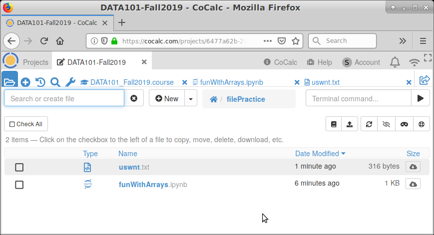
Figure \(\PageIndex{1}\): A directory (folder) on CoCalc, which contains two files: a plain-text file (called uswnt.txt) and a Jupyter Notebook which will read from it (funWithArrays.ipynb).

The two entries listed are a plain-text file (called uswnt.txt) and a Jupyter Notebook (funWithArrays.ipynb). You can tell that the former is a plain-text file because of the filename extension “.txt”.⁸ If we clicked on uswnt.txt, we’ll bring up the contents of the file, as shown in Figure 8.2.2. In this case, we have the current roster on the US Women’s National Soccer team, one name per line. Perhaps the most important thing to see is that the file itself, which we will read into Python in a moment, is nothing strange or scary: you could type it yourself into Notepad or Word.⁹

This is a good time to mention that spaces and other funny characters in filenames are considered evil. You might think it looks better to call the notebook file “fun with arrays.ipynb” and the data file “US Women’s National Team roster.txt”, but I promise you it will lead to pain in the end, for a variety of fiddly reasons. It’s better to use camel case for filenames, which is simply capitalizingEachSuccessiveWordInAPhrase.

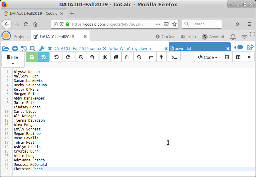
Figure \(\PageIndex{2}\): The contents of a plain-text file, as rendered by CoCalc.

Okay, finally back to NumPy code. If all the stars are aligned, we can write this code in a funWithArrays.ipynb cell to read the soccer roster into an ndarray:

Code \(\PageIndex{5}\) (Python):

roster = np.loadtxt("uswnt.txt", dtype=object, delimiter="###")

There’s a lot of weird stuff in that line, so follow me here. The first argument is easy enough: the name of the file that contains our data. (Again, I stress that the file must be located in the same directory as the notebook!) The second argument is bizarre: we know what dtype means, but “object”? Ugh, another fiddly detail. When you read from a file into a NumPy array, you will be reading one of our three atomic types. Here are the rules:

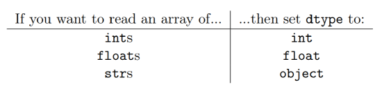
So basically, you set dtype to the type of data you want in your ndarray...unless you want strings, in which case you put the word object. Sorry about that.

The last of the three arguments is even nuttier, and you actually don’t need to include it at all if you’re reading ints or floats. If you’re reading strs, however, you need to set the delimiter to something that doesn’t appear in any of the strs. I chose three-hashtags-in-a-row since that rarely appears in any set of text data.

Bottom line: once we’ve done all this, we get:

Code \(\PageIndex{6}\) (Python):

print(roster)

| ['Alyssa Naeher' 'Mallory Pugh' 'Sam Mewis' 'Becky Sauerbrunn' "Kelly O'Hara" 'Morgan Brian' 'Abby Dahlkemper' 'Julie Ertz' 'Lindsey Horan' 'Carli Lloyd' 'Ali Krieger' 'Tierna Davidson' 'Alex Morgan' 'Emily Sonnett' 'Megan Rapinoe' 'Rose Lavelle' 'Tobin Heath' 'Ashlyn Harris' 'Crystal Dunn' 'Allie Long' 'Adrianna Franch' 'Jessica McDonald' 'Christen Press']

which is pretty cool.

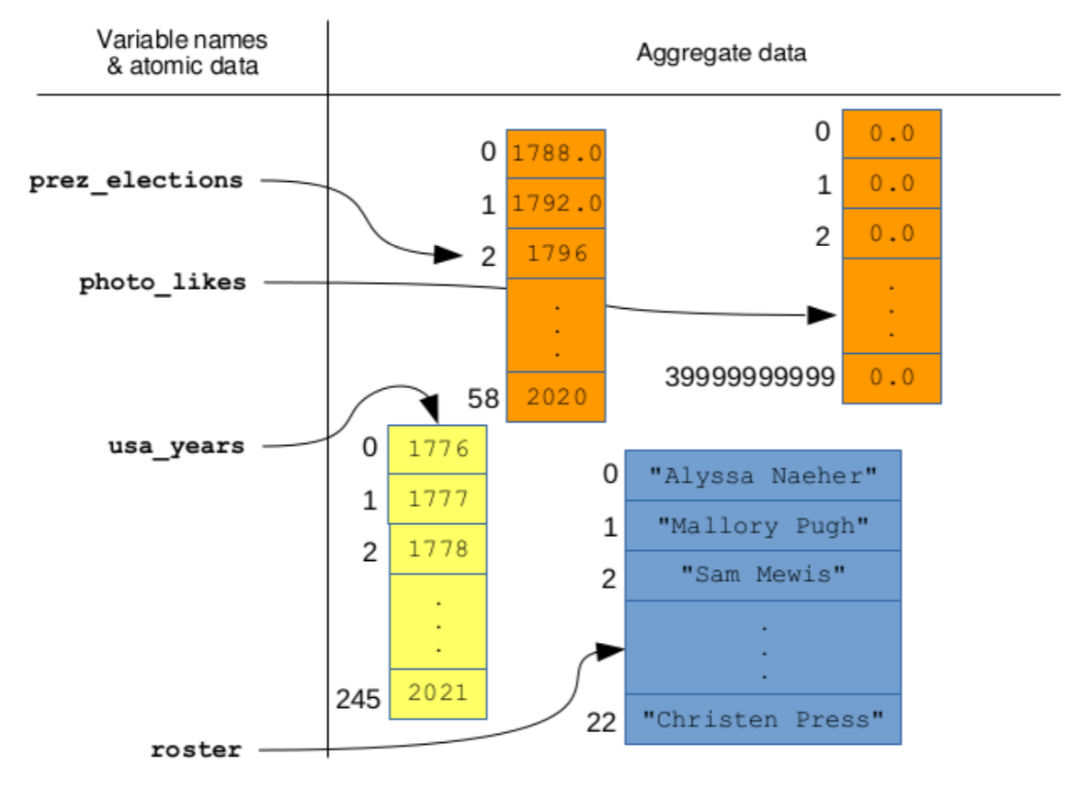
Figure \(\PageIndex{3}\): The memory picture of the four arrays we created in section 8.2.