15.2: Numerical data- Quantiles

A quantile is a real number between 0 and 1 that represents a “cut point” of a numerical data set: roughly speaking, it’s the number for which a certain fraction of the values are less than that number. So the “.2-quantile” (pronounced “point two quantile”) of a variable containing the heights of third-graders might be 50 inches. If that’s the case, it would indicate that 20% of the third-graders are less than 50 inches tall.

Quantiles are very revealing, but underappreciated. Most people don’t seem to know how to interpret them. But once you figure it out, you’ll realize that quantiles tell you almost everything possible to know about a numeric variable: by dialing the quantile between 0 and 1, you can tell exactly how common values in certain ranges are.

In Python, you simply call the .quantile() method on a Series, passing a number between 0 and 1 as an argument, and it tells you exactly where that cut point is.

Now there’s a little bit of weirdness around the edges, depending on the exact definition used to calculate the quantiles. Let’s say I collected some salary data, and got these responses (“k” means “thousand dollars per year,” and “M” means “million dollars per year”):

35k 22k 67k 45k 35k 8M 94k 51k 53k 64k 54k

How would I calculate, say, the .7-quantile? First, sort the numbers:

22k 35k 35k 45k 51k 53k 54k 64k 67k 94k 8M

(yes, we do include the 35k value twice; don’t eliminate duplicates) and then spread out the quantiles “evenly” from 0 to 1:

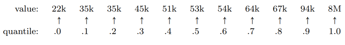
Don’t get picky on me. If you were picky, you could quibble at saying “the .3-quantile is 45k” since it’s technically not true that 30% of the values are less than 45k: in truth, 3 out of 11 (27.3%) of them are. Whatever, whatever. The point is that 45k is at the “cut point” that’s 3 10 ths of the way through the values from min to max. Quantiles aren’t about laser precision anyway: they’re about understanding the general pattern of the data.

“Special” quantiles

You’ll realize as an immediate consequence of the above that the median is just another name for the .5-quantile. It’s the value for which half the data points are below it, and half above. Also, the 0-quantile is just the minimum of the data set, and the 1-quantile the maximum.

Other kinds of “-tiles”

This whole idea may ring bells with other names for you: quartiles, quintiles, deciles, or (most probably) percentiles. All of those are basically special cases of quantiles. They split the data into evenly-sized groups:

• “quartiles”: split the data into four groups, with the split points being the .25-, .5-, and .75-quantiles.
• “quintiles”: split the data into five groups, with the split points being the .2-, .4-, .6, and .8-quantiles.
• “deciles”: split the data into ten groups, with the split points being the .1-, .2-, .3-, .4-, .5-, .6-, .7-, .8-, and .9-quantiles.
• “percentiles”: split the data into 100 groups, with the split points being the .01-, .02-, .03-, ..., .98-, and .99-quantiles.

Be careful to understand that “evenly-sized groups” does not mean “groups with the same-sized range,” but rather “groups with the same number of data points in them.” Normally, in fact, the ranges will not be the same size. The lowest quintile for a data set of IQs might range from 47 (the lowest IQ in the data set) all the way up to 83, whereas the IQs in the middle quintile might all be in the narrow range 96 to 104.

The IQR (interquartile range)

Speaking of quartiles, you’ll commonly hear data scientists cite the IQR, or interquartile range, as a measure of how widely varying a univariate data set is. It’s simply the distance between the .25- quantile and the .75-quantile; or in quartile terms, the difference between the “upper” and “lower” quartiles.

Because of how quantiles work, exactly 50% of the data points are between the .25- and .75-quantiles. This means that the more spread out the data points are, the larger the IQR, and vice versa. In this sense, it’s akin to the standard deviation (see p. 153) which you may be familiar with.

A quantile example

Let’s nail this down with an example. I have a (fictitious) data set containing the number of YouTube plays for each of a selection of videos. It’s called num_plays. Here are the first few values:

| 0 791

| 1 3133

| 2 0

| 3 1789

| 4 297

| 5 219

| 6 1688

| 7 209

| 8 422

| 9 91454

| dtype: int64

That’s great, but it’s both too much information and too little: we can pore through the plays for every single video, but it’s hard to get our head around what the overall contents are. So let’s run some quantiles. We’ll start with the .1-quantile:

Code \(\PageIndex{1}\) (Python):

print(num_plays.quantile(.1))

Whoa. The .1-quantile is zero. Think about what that means. Pictorially, sorting the data would give this:

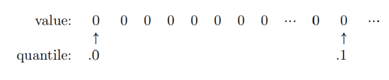
Put another way, that means that (at least) 10% of our videos have no plays at all.

Let’s try the .2-quantile:

Code \(\PageIndex{2}\) (Python):

print(num_plays.quantile(.2))

Okay, now at least we have a pulse. But in case we thought this was data set was packed with big hits, think again: a full 20% of these videos have fewer than 15 plays.

The median is:

Code \(\PageIndex{3}\) (Python):

print(num_plays.quantile(.5))

That’s quite a bit higher. How about the 90% mark?

Code \(\PageIndex{3}\) (Python):

print(num_plays.quantile(.9))

| 1378.0

All right, so the upper end of these videos are in the thousands. Finally, let’s look at the max:

Code \(\PageIndex{4}\) (Python):

print(num_plays.quantile(1))

!!

Believe it or not, this sort of thing isn’t unusual, especially with data from social phenomena. The tiny fraction of the data at the upper end of the range is vastly higher than everything else is. Get your head around that: the median number of plays was a couple hundred, but the maximum number of plays was nearly a million.

Computing the IQR of this data set is as simple as finding the difference between the .25 and .75 quantiles:

Code \(\PageIndex{5}\) (Python):

print(num_plays.quantile(.75) - num_plays.quantile(.25))