
8: Accelerated Performance - Turns
- Page ID
- 75453

\( \newcommand{\vecs}[1]{\overset { \scriptstyle \rightharpoonup} {\mathbf{#1}} } \)
\( \newcommand{\vecd}[1]{\overset{-\!-\!\rightharpoonup}{\vphantom{a}\smash {#1}}} \)
\( \newcommand{\dsum}{\displaystyle\sum\limits} \)
\( \newcommand{\dint}{\displaystyle\int\limits} \)
\( \newcommand{\dlim}{\displaystyle\lim\limits} \)
\( \newcommand{\id}{\mathrm{id}}\) \( \newcommand{\Span}{\mathrm{span}}\)
( \newcommand{\kernel}{\mathrm{null}\,}\) \( \newcommand{\range}{\mathrm{range}\,}\)
\( \newcommand{\RealPart}{\mathrm{Re}}\) \( \newcommand{\ImaginaryPart}{\mathrm{Im}}\)
\( \newcommand{\Argument}{\mathrm{Arg}}\) \( \newcommand{\norm}[1]{\| #1 \|}\)
\( \newcommand{\inner}[2]{\langle #1, #2 \rangle}\)
\( \newcommand{\Span}{\mathrm{span}}\)
\( \newcommand{\id}{\mathrm{id}}\)
\( \newcommand{\Span}{\mathrm{span}}\)
\( \newcommand{\kernel}{\mathrm{null}\,}\)
\( \newcommand{\range}{\mathrm{range}\,}\)
\( \newcommand{\RealPart}{\mathrm{Re}}\)
\( \newcommand{\ImaginaryPart}{\mathrm{Im}}\)
\( \newcommand{\Argument}{\mathrm{Arg}}\)
\( \newcommand{\norm}[1]{\| #1 \|}\)
\( \newcommand{\inner}[2]{\langle #1, #2 \rangle}\)
\( \newcommand{\Span}{\mathrm{span}}\) \( \newcommand{\AA}{\unicode[.8,0]{x212B}}\)
\( \newcommand{\vectorA}[1]{\vec{#1}} % arrow\)
\( \newcommand{\vectorAt}[1]{\vec{\text{#1}}} % arrow\)
\( \newcommand{\vectorB}[1]{\overset { \scriptstyle \rightharpoonup} {\mathbf{#1}} } \)
\( \newcommand{\vectorC}[1]{\textbf{#1}} \)
\( \newcommand{\vectorD}[1]{\overrightarrow{#1}} \)
\( \newcommand{\vectorDt}[1]{\overrightarrow{\text{#1}}} \)
\( \newcommand{\vectE}[1]{\overset{-\!-\!\rightharpoonup}{\vphantom{a}\smash{\mathbf {#1}}}} \)
\( \newcommand{\vecs}[1]{\overset { \scriptstyle \rightharpoonup} {\mathbf{#1}} } \)
\(\newcommand{\longvect}{\overrightarrow}\)
\( \newcommand{\vecd}[1]{\overset{-\!-\!\rightharpoonup}{\vphantom{a}\smash {#1}}} \)
\(\newcommand{\avec}{\mathbf a}\) \(\newcommand{\bvec}{\mathbf b}\) \(\newcommand{\cvec}{\mathbf c}\) \(\newcommand{\dvec}{\mathbf d}\) \(\newcommand{\dtil}{\widetilde{\mathbf d}}\) \(\newcommand{\evec}{\mathbf e}\) \(\newcommand{\fvec}{\mathbf f}\) \(\newcommand{\nvec}{\mathbf n}\) \(\newcommand{\pvec}{\mathbf p}\) \(\newcommand{\qvec}{\mathbf q}\) \(\newcommand{\svec}{\mathbf s}\) \(\newcommand{\tvec}{\mathbf t}\) \(\newcommand{\uvec}{\mathbf u}\) \(\newcommand{\vvec}{\mathbf v}\) \(\newcommand{\wvec}{\mathbf w}\) \(\newcommand{\xvec}{\mathbf x}\) \(\newcommand{\yvec}{\mathbf y}\) \(\newcommand{\zvec}{\mathbf z}\) \(\newcommand{\rvec}{\mathbf r}\) \(\newcommand{\mvec}{\mathbf m}\) \(\newcommand{\zerovec}{\mathbf 0}\) \(\newcommand{\onevec}{\mathbf 1}\) \(\newcommand{\real}{\mathbb R}\) \(\newcommand{\twovec}[2]{\left[\begin{array}{r}#1 \\ #2 \end{array}\right]}\) \(\newcommand{\ctwovec}[2]{\left[\begin{array}{c}#1 \\ #2 \end{array}\right]}\) \(\newcommand{\threevec}[3]{\left[\begin{array}{r}#1 \\ #2 \\ #3 \end{array}\right]}\) \(\newcommand{\cthreevec}[3]{\left[\begin{array}{c}#1 \\ #2 \\ #3 \end{array}\right]}\) \(\newcommand{\fourvec}[4]{\left[\begin{array}{r}#1 \\ #2 \\ #3 \\ #4 \end{array}\right]}\) \(\newcommand{\cfourvec}[4]{\left[\begin{array}{c}#1 \\ #2 \\ #3 \\ #4 \end{array}\right]}\) \(\newcommand{\fivevec}[5]{\left[\begin{array}{r}#1 \\ #2 \\ #3 \\ #4 \\ #5 \\ \end{array}\right]}\) \(\newcommand{\cfivevec}[5]{\left[\begin{array}{c}#1 \\ #2 \\ #3 \\ #4 \\ #5 \\ \end{array}\right]}\) \(\newcommand{\mattwo}[4]{\left[\begin{array}{rr}#1 \amp #2 \\ #3 \amp #4 \\ \end{array}\right]}\) \(\newcommand{\laspan}[1]{\text{Span}\{#1\}}\) \(\newcommand{\bcal}{\cal B}\) \(\newcommand{\ccal}{\cal C}\) \(\newcommand{\scal}{\cal S}\) \(\newcommand{\wcal}{\cal W}\) \(\newcommand{\ecal}{\cal E}\) \(\newcommand{\coords}[2]{\left\{#1\right\}_{#2}}\) \(\newcommand{\gray}[1]{\color{gray}{#1}}\) \(\newcommand{\lgray}[1]{\color{lightgray}{#1}}\) \(\newcommand{\rank}{\operatorname{rank}}\) \(\newcommand{\row}{\text{Row}}\) \(\newcommand{\col}{\text{Col}}\) \(\renewcommand{\row}{\text{Row}}\) \(\newcommand{\nul}{\text{Nul}}\) \(\newcommand{\var}{\text{Var}}\) \(\newcommand{\corr}{\text{corr}}\) \(\newcommand{\len}[1]{\left|#1\right|}\) \(\newcommand{\bbar}{\overline{\bvec}}\) \(\newcommand{\bhat}{\widehat{\bvec}}\) \(\newcommand{\bperp}{\bvec^\perp}\) \(\newcommand{\xhat}{\widehat{\xvec}}\) \(\newcommand{\vhat}{\widehat{\vvec}}\) \(\newcommand{\uhat}{\widehat{\uvec}}\) \(\newcommand{\what}{\widehat{\wvec}}\) \(\newcommand{\Sighat}{\widehat{\Sigma}}\) \(\newcommand{\lt}{<}\) \(\newcommand{\gt}{>}\) \(\newcommand{\amp}{&}\) \(\definecolor{fillinmathshade}{gray}{0.9}\)Introduction
Historical Introduction
Thus far all of our performance study has involved straight line flight. Unfortunately, unless our airplane is flying from a runway that is exactly in line with our destination runway and there is no wind on the route, straight line flight isn’t very practical! We need to be able to turn.
While the need to be able to turn is fairly obvious to us, a look at early aviation will show that it often was the last thing on the mind of many aviation pioneers. The uniqueness of the Wright Flyer was not its ability to fly a few feet in a straight line over the sand at Kitty Hawk. It was unique in its ability to turn and maneuver. There are claims that earlier experimenters in England, France, Russia, and the United States may indeed have made short, uncontrolled “hops” or even legitimate straight line “flights” in powered vehicles before December 17, 1903 but there are no claims for “controlled” flight of a powered, heavier than air, man (or woman) carrying vehicle prior to this date.
There are several ways to turn a vehicle in flight. Early experimenters such as Otto Lilienthal in Germany and Octave Chanute in this country knew that shifting the weight of the “pilot” suspended beneath their early “hang gliders” would tilt or “bank the wings to allow turns. Others such as Samuel P. Langley, the turn of the century director of the Smithsonian who had government funding to build and fly the first airplane, designed their craft to be steered with a rudder like a ship. Neither method of turning was very efficient. Langley’s heavier than air powered models, for example, flew very well but couldn’t adjust for winds and flew in long circles instead of a straight line as they had been designed to do.
Banking the wings (called the “aero‑planes” in the 1890’s) tilts the lift force to the side and the sideward component of the lift results in a turn, but since part of the lift is now being used to turn the vehicle the remaining lift may not be enough to oppose the weight unless additional power is added. Using a rudder alone results in a side force on the fuselage of the aircraft and, hence, a turning force. The resulting turn, by causing one wing to move forward faster than the other, usually leads to a bank. Neither method, employed alone, provides a very satisfactory means of turning and the result is usually a very large radius turn. Many early experimenters, in fact, appeared to want to turn without banking since they were “flying” very close to the ground and a banked wing might touch the ground and cause a crash.
The Wright brothers designed a complex mechanism involving coordinated rudders and twisting of wings to combine both roll and yaw in a “coordinated”, efficient turn. Their original purpose may have actually been to try to bank the airplane opposite the turn to prevent ground contact by the wing but they found that a properly coordnated turn could make their vehicle quite maneuverable. When the Wrights took their aircraft to Europe in 1908 they amazed European aviators with their craft’s ability to turn and maneuver. French airplanes, which were the most sophisticated in Europe, used only rudders to turn. The Wright Flyer, with its “wing warping” system and coordinated rudder, was literally able to fly circles around the French aircraft.
The Wrights had made this system of ropes and pulleys which connected rudder to twisting wing tips to a cradle under the pilot’s body, the central focus of their patent on the airplane. When world motorcycle high speed record holder and engine designer Glenn Curtiss, with funding from Alexander Graham Bell and others, built and flew an airplane with performance as good as or better than the Wright Flyer, the Wrights sued for patent violation. The Curtiss planes, which used either small, separate wings near the wing tips or wingtip mounted triangular flaps (later to be called ailerons) and which relied on pilot operation of separate controls like today’s stick and rudder system, were able to achieve the same turning performance as the Wrights Flyer. Curtiss, a much more flamboyant and public figure than either of the Wrights, quickly captured the attention and imagination of the American public, infuriating the Wrights who had shunned public attention while convincing themselves that no one else was capable of duplicating their aerial feats.
The decade long court battle between Curtiss and the Wright family over patent rights to devices capable of efficiently turning an airplane is credited by most historians as allowing European aviators and designers to forge far ahead of Americans. The Wrights were so absorbed with protecting their patent that they made no further efforts to improve the airplane and the threat of a Wright lawsuit kept all American airplane designers but Curtiss out of the business. Curtiss, whose lack of respect for caution had earlier enabled him to set the world motorized speed record on a motorcycle with a V‑8 engine, with moral and financial support from Bell and Henry Ford and others, kept the patent suit in court through appeal after appeal and continued to build and sell airplanes. To get around the Wright patent, Curtiss, at one time built his aircraft without ailerons or other roll controls and then shipped them to nearby Canada where one of Bell’s companies added the ailerons before the planes were shipped to customers in Europe! Meanwhile, Curtiss continued to experiment and innovate and it is no accident that when the first World War drew American participation it was Curtiss and not Wright aircraft that went to war. After the war it was the famed Curtiss “Jenny” that brought the “barnstorming” age of aviation to all America.
I hope the reader will pardon the above slip into historical fascination. By now some of you are asking what the heck all of this has to do with aircraft performance in turns? The facts are, however, that the first ten to fifteen years of American flight really were dominated by the airplane’s ability to turn.
8.1 The Mechanics of a Turn
To keep the physics of our discussion as simple as possible, lets consider only turns at constant radius in a horizontal plane. This is the ideal turn with no loss or gain of altitude which every student pilot practices by flying in circles around some farmer’s silo or other prominent landmark.
Our objectives in looking at turning performance will be to find things like the maximum rate of turn and the minimum turning radius and to determine the power or thrust needed to maintain such turns. We will begin by looking at two types of turns.
Today’s airplanes, in general, make turns using the same techniques pioneered by the Wrights and improved by Curtiss; coordinated turns using rudder and aileron controls to combine roll and yaw. The primary exception would be found in some evasive turning maneuvers made by military aircraft and in the everyday turns of most student pilots!
Non‑winged vehicles such as missiles, airships, and submarines still make turns like those of early French aviators and of Langleys “Aerodrome”, using rudder and body or fuselage sideforce to generate a “skiding” turn. We will examine this technique before looking at the more sophisticated coordinated turn.
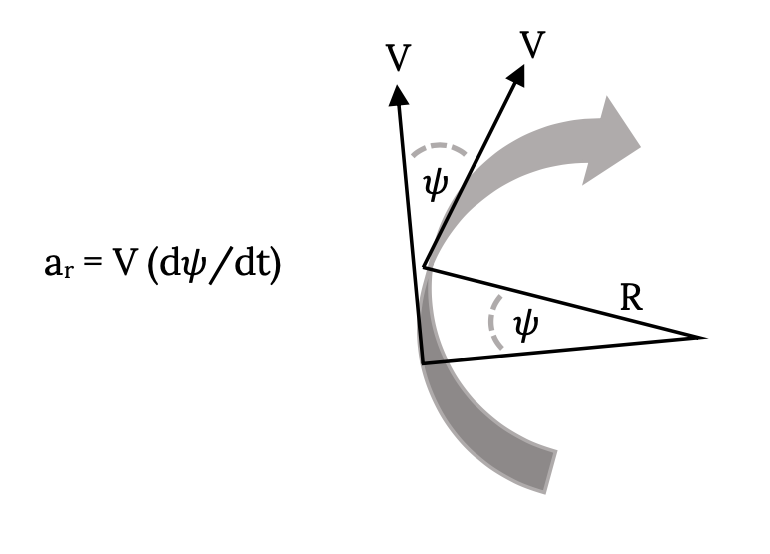
The acceleration in any turn of radius \(R\) is given by the following relation:
\[a_r = \dfrac{V^2}{R}. \nonumber\]
This acceleration is directed radially inward toward the center of the circle and is properly termed the centripital acceleration.
We can also consider the acceleration from the perspective of the rate of change of the “heading angle”, ψ, as shown in the figure below.
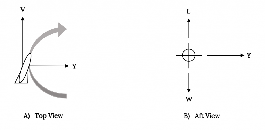
The “skid to turn” technique is illustrated below for a constant radius, horizontal turn. A rudder (or even vectored thrust) is used to angle the vehicle and the sideforce created by the flow over the yawed body creates the desired acceleration.
The equations of motion become
L – W = 0
Y = mV(dψ/dt) = m(V2/R)
For the skid turn examined above, the turning rate and radius depend on the amount of side force which can be generated on the body of the vehicle. Note that the lift (or buoyancy in the cases of submarines and airships) does not enter into the problem.
R = (WV2)/(gY) , dψ/dt = (gY)/(WV)
With the above relationships one can determine the radius and rate for a horizontal turn where body force, not wing lift, carries the vehicle through a turn. This is how non-winged rockets and missiles turn. Airplanes use a much more powerful force, the lift, to turn. By using the lift to provide the needed sideforce and to counteract the weight in a coordinated fashion an airplane can make a much more efficient turn than missiles or dirigibles.
Let’s look at the coordinated turn. In the ideal coordinated turn as illustrated in Figure 8.3, the aerodynamic lift is used to balance the weight such that horizontal flight is maintained and to provide a side force which produces the desired turning acceleration. No actual side force is generated on the fuselage of the aircraft. This type of turn requires the pilot to use the rudder and the ailerons and the throttle to give the ideal balance of bank angle and forces which will create a constant radius turn and maintain altitude.
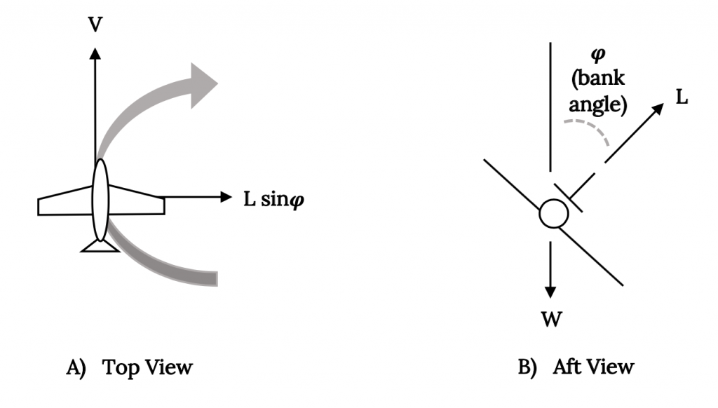
If this turn is properly coordinated the resulting combined acceleration and gravitational force felt by both airplane and pilot will be directed “down” along the vertical axis of the aircraft and will be felt by the pilot as an increased force into the seat. The improperly coordinated will be felt as including a side force pushing the pilot left or right in the seat. These same forces act on the “ball” in the aircraft’s “turn‑slip” indicator, moving the ball off center in an uncoordinated turn. We will look at the turn-slip indicator later.
If a turn is not coordinated several results may occur. The turning radius will not be constant and the airplane will either “skid” outward to a larger radius turn or “slip” inward to a smaller radius. There could also be a gain or loss of altitude.
In the coordinated turn, part of the lift produced by the wing is used to create the turning acceleration. The remainder of the lift must still counteract the weight to maintain horizontal flight.
We now find ourselves looking for the first time at a situation where lift is not equal to weight. In a coordinated turn the lift must be greater than the weight and we define a “load factor”, n, to account for this inequality.
\[L = nW\]
This load factor can then be related to the bank angle used in the turn, to the turn radius, and to the rate of turn. Returning to the vertical force balance equation we have
\[\mathbf{L} \cos \varphi-\mathbf{W}=\mathbf{n} \mathbf{W} \cos \varphi-\mathbf{W}=\mathbf{0}\]
which gives:
\[\cos \varphi=1 / \mathrm{n}\]
Using the other equation of motion we can find the turn radius
\[\mathbf{R}=\left(\mathbf{m} \mathbf{V}^{2}\right) /(\mathbf{L} \sin \varphi)=\left(\mathbf{m} \mathbf{V}^{2}\right) /(\mathbf{n} \mathbf{W} \sin \varphi)=\left(\mathbf{V}^{2} / \mathbf{n g}\right)(\mathbf{1} / \sin \varphi)\]
Knowing that the cosine of the bank angle is equal to 1/n we can find the value of the sine of the bank angle by constructing a right triangle
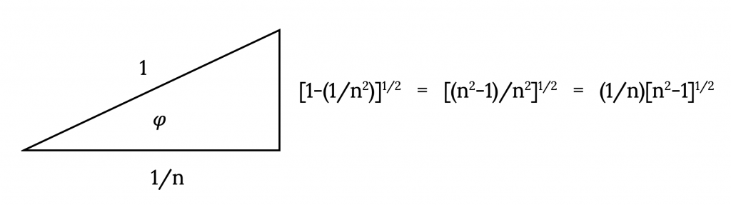
hence,
/n2]1/2andtanφ=[n2−1]1/2")
and the turning radius becomes
R = (V2/g){ 1 / [n2 – 1]1/2} .
In dealing with turns we must remember that lift is no longer equal to weight. The lift coefficient is then
=(2nW)/(ρV2S)")
therefore
/(ρSCL)")
The above allows us to write the turning radius in another manner,
][n/(n2−1)1/2]")
It should be noted here that if a small turning radius is desired a high load factor and lift coefficient are needed and low altitude will help. High wing loading (W/S) will also allow a tighter turn.
The rate of turn in a coordinated turn is
/(mV)={(nmg)/(mV)}sinφ=[ng/V][(n2−1)1/2/n]")
or
[n2−1]1/2")
Alternatively,
/(2W)]1/2[(n2−1)/n]1/2}")
The same factors which contribute to small turning radii give high rates of turn.
8.2 Load factor (n)
From the above equations it is obvious that the load factor plays an important role in turns. In straight and level flight the load factor, n, is 1. In maneuvers of any kind the load factor will be different than 1. In a turn such as those described it is obvious that n will exceed 1. The same is true in maneuvers such as “pull ups”.
The load factor is simply a function of the amount of lift needed to perform a given maneuver. If the required bank angle for a coordinated turn is 60° the load factor must equal 2. This means that the lift is equal to twice the weight of the aircraft and that the structure of the aircraft must be sufficient to carry that load. It also means that the pilot and passengers must be able to tolerate the loading imposed on them by this turn, a load which is forcing their body into their seat with an effect twice that of normal gravity. This “2g” load or acceleration is also forcing their blood from their heads to their feet and having other interesting effects on the human body.
If we look at the lift relation
L = nmaxW = CLmax[½ρV2S]
we see that the maximum lift and therefore the maximum load factor that may be generated aerodynamically is a function of the maximum lift coefficient (stall conditions).
One must realize that the aircraft, or, more precisely, its wings, may be capable of generating far higher load factors than either the pilot and passengers or the aircraft structure may be able to tolerate. It is not hard to design aircraft which can tolerate far higher “g‑loads” than the human body, even when the body is in a prone position in a specially designed seat and uniform. Engineers in the industry will tell you that they could design far more agile fighters at much lower cost if the military didn’t insist on having pilots in the cockpit!
All aircraft, from a Cessna 152 to the X‑31, are designed to tolerate certain load factors. The aerobatic version of the Cessna 152 is certified to tolerate a higher load factor than the “commuter” version of that aircraft. An aerobatic aircraft must be designed for a load factor of 6.
The FAA also imposes certain flight restrictions on commercial aircraft based on passenger comfort. It is possible to do aerobatics in a Boeing 777 but most of the passengers wouldn’t like it. Passenger carrying commercial flight is therefore normally restricted to “g‑loads” of 1.5 or less even though the aircraft themselves are capable of much more.
8.3 The two-minute turn
General aviation pilots are usually familiar with the “standard rate” or “two‑minute” turn. This turn, at a rate of three‑degrees per second (0.05236 rad/sec), is used in maneuvers under controlled instrument flight conditions. To make such a turn the pilot uses an instrument called a “turn‑slip” indicator. This instrument, illustrated below, consists of a gyroscope which is partially restrained and attached to a needle indicator, and a curved tube containing a ball in white kerosene. As the airplane turns, the gyroscope deflects the indicator needle as it attempts to remain fixed in orientation. The “precession” force of the gyroscope and the resulting needle displacement is proportional to the turn rate. The accuracy of this indication is not dependent on the degree to which the turn is coordinated. The ball in the curved tube will stay centered if the turn is coordinated while it will move to the side (right or left) if it is not coordinated. One of the sets of markings on the face of the instrument indicates a two minute turn.
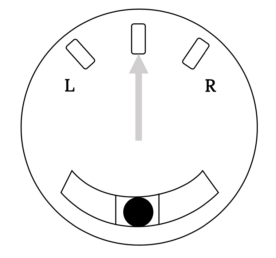
8.4 The Turn-Slip Indicator
To make a two‑minute turn the pilot need only place the aircraft in a turn such that the needle is at the standard turn indication in the desired direction. To turn 90º the turn rate is maintained for 30 seconds, one minute for 180º, etc. The vertical speed indicator (rate of climb) is used to maintain altitude and the ball is kept centered to coordinate the turn.
Many pilots are taught, incorrectly, that the two‑minute turn mark on the turn-slip indicator is an indication of a 15 degree bank angle, with the next mark being 30º and so on. Some pilots even refer to the turn‑slip indicator as the “turn‑bank” indicator when the instrument has absolutely no way to detect bank. It is possible, using a “cross control” technique, to turn the aircraft via yaw with no bank (much like a missile turns) and see that the instrument indicates the correct rate of turn even though there is no bank and, similarly, the aircraft may be placed in roll without turning and the indicator will remain centered.
Why would this error in flight instruction occur? The answer lies partly in the difficulty in eradicating longstanding lore and partly in the fact that, for a small general aviation trainer airplane, a coordinated two‑minute turn does occur at about a 15 degree bank angle. Let’s look at the numbers.
From our previous equations we have
dψ/dt")
Inserting fifteen degrees as the bank angle and a two minute turn rate (0.05236 rad/sec) gives a velocity of 165 ft/sec or 112 mph. This is indeed close to the speed at which such an airplane would fly in a turn. If we, however, look at a faster aircraft, lets say one that is operating at 350 miles per hour, and use the two‑minute rate of turn we get a very different bank angle of 30 degrees!
Suppose you are a passenger in a Boeing 737 traveling at 600 mph and the pilot set up a two minute turn. This would give a bank angle of 55 degrees. It would also give a load factor of 1.75! This is higher than the FAA allows for airline operations. For this reason airliners use turn rates slower than the two minute turn in flight and only make two minute turns at low speeds, perhaps when operating in the “pattern” around airports.
8.5 Instantaneous versus sustained turn conditions
The previously derived relations will give the instantaneous turn rate and radius for a given set of flight conditions. In other words, for a given set of initial flight conditions we can determine the turn rate and radius, etc. Another question which must be asked is “Can the airplane sustain that turn rate?” The pilot may be able to, for example, place the plane in a 60 degree bank at 250 mph but may find that there is not enough engine thrust to hold that speed and bank angle while maintaining altitude.
For the airplane with the specifications below find the maximum turn rate and minimum radius of turn and the speeds at which they occur. Also determine if this turn can be sustained at sea level standard conditions.
W/S = 59.88 lb/ft2
S = 167 ft2
CLmax = 1.5
nmax = 6
CD0 = 0.018
K = 0.064
Tmax = 5000 lb
The maximum turning rate is
/(2W)]1/2[(nmax2−1)/nmax]1/2")
= 0.424 rad/sec = 24.29 o/sec .
The velocity for this turn rate is
/(ρSCLmax)]1/2=448.6ft/sec")
The minimum turning radius is
][n/(n2−1)1/2]=1058ft=V/[dψ/dt]")
Now we must see if the plane has enough thrust to operate at these conditions. The drag coefficient at maximum lift coefficient is
CD = 0.018 + 0.064 CLmax2 = 0.162 .
At the speed found above the drag is then
=6479lb")
This drag exceeds the thrust available from the aircraft engine!
If the above aircraft enters a coordinated turn at the maximum turn rate it will quickly slow to a lower speed and turning rate with a larger turn radius or it will lose altitude.
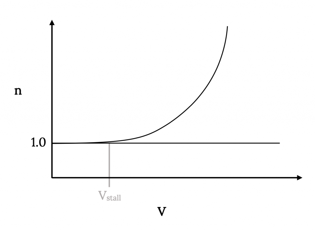
8.6 The V‑n or V‑g Diagram
A plot which is sometimes used to examine the combination of aircraft structural and aerodynamic limitations related to load factor is the V‑n or V‑g diagram. This is a plot of load factor n versus velocity.
We know that when lift exceeds weight
")
We know that one limit is imposed by stall
")
Rearranging this we can write
")
and we can rearrange this as
]1/2")
Plotting n versus V will then give a curve like that shown below.
We can also consider negative load factors which will relate to “inverted” stall; ie, stall at negative angle of attack. At negative angle of attack, unless the wing is untwisted and constructed of symmetrical airfoil sections, CLmax will be different from that at positive angle of attack. This will give a different but similar curve below the axis. Combining this with the plot above gives the following plot.
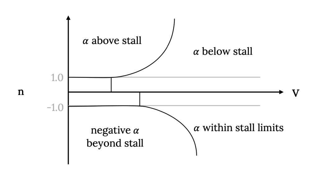
To the left of this curve is the post‑stall flight region which, with the exception of high performance military aircraft, represents a out‑of‑bounds area for flight.
Other limits must also be considered. There will obviously be an upper speed limit such as that found earlier for straight and level flight. There will also be limits imposed by the structural design of the aircraft. Depending on the aircraft’s structural category (utility, aerobatic, etc.) it will be designed to structurally absorb load factors up to a given limit at positive angle of attack and another limit at negative angle of attack. Once these are defined, the complete V‑n diagram denotes an operating envelope in terms of load factor limits.
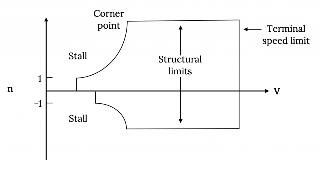
The point where the structural limit line and the stall limit intersect is termed a “corner point”. The velocity at this point is limited by both maximum structural load factor and CLmax. The velocity at that point is
/(ρCLmaxS)]1/2")
At speeds below the “corner velocity” it is impossible to structurally damage the airplane aerodynamically because the plane will stall before damage can occur. At speeds above this value it is possible to place the aircraft in a maneuver which will result in structural damage, provided the plane has sufficient thrust to reach that speed and load.
It is possible for a wind “gust” to cause loads which exceed the above limits. Such gusts may be part of what is referred to as wind shear and are common around thunderstorms or mountain ridges. Gusts can be in either the vertical or horizontal direction. The primary effect of a horizontal gust is to increase or decrease the likelihood of stall due to the change in speed relative to the wing. This is often the cause of wind shear accidents around airports where the aircraft is operating at near-stall conditions.
If a gust is vertical, we can look at its effect in terms of change of angle of attack. Suppose we have a vertical gust of magnitude wg. Its effect on the angle of attack and CL is seen below.
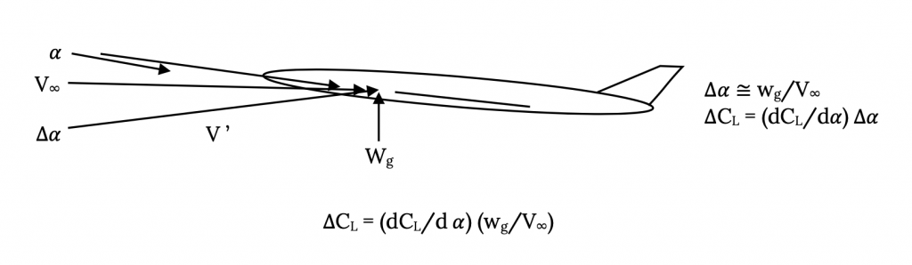
so the change in lift is
Thus
If, for example, an aircraft in straight and level flight encounters a vertical gust of magnitude wg the new load factor is
(for straight and level flight n = 1)
The effect of the gust on the load factor is therefore amplified by the flight speed V. This effect can be plotted on the V‑n diagram to see if it results in stall or structural failure.
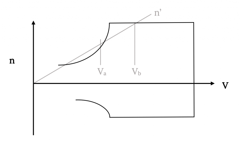
For the case illustrated above, the gust will cause stall if it occurs at a flight speed below Va and can cause structural failure if it occurs at speeds above Vb.
Homework 8
We wish to compare the performance of two different types of “General Aviation” aircraft; the popular Cessna Citation III business jet and the best all-around, four place, single engine, piston plane in the business, the Cessna 182. Approximate aerodynamic and performance characteristics are given in the table below:
Table 8.1: Aerodynamic and Performance Characteristics
| CITATION III | CESSNA 182 | |
|---|---|---|
| Wingspan | 53.3 ft | 35.8ft |
| Wing area | 318 ft^2 | 174 ft^2 |
| Normal gross weight | 19,815 lb | 2,950 lb |
| Total thrust at sea level | 7300 lb | --------- |
| Usable power at sea level | --------- | 230 hp |
| C_D0 | 0.02 | 0.025 |
| Oswald Efficiency Factor (e) | 0.81 | 0.80 |
1. Calculate and tabulate the thrust required (drag) versus Ve data for both aircrafts and plot the results on the same graph [Figure 8.11]. Plot the sea level thrust available curves for both aircrafts on the same graph [Figure 8.11].
2. Calculate the maximum velocity at sea level for both aircraft and compare with that indicated on the graph [Figure 8.11].
3. Calculate and tabulate the power required versus Ve data for both aircraft and plot each on a separate graph [Figures 8.12 and 8.13]. Plot the sea level power available on the same graphs.
Figure 8.12: Power at Sea Level For Prop
4. Calculate and tabulate the rate of climb (in ft/min) versus velocity data at sea level for both aircraft for normal gross weight and plot the data on the same graph [Figure 8.14].
Figure 8.14: Rate of Climb at Sea Level for Citation III and C-182
5. Calculate and tabulate the maximum rate of climb versus altitude data for both aircraft and plot it on the same graph. [Figure 8.15]. Determine the absolute ceilings of both aircraft.
6. Calculate the time required to climb from sea level to 20,000 ft for both aircraft. Assume that the curves (in 5) are close enough to linear to use a linear approximation for the calculation.
References
Figure 8.1: Kindred Grey (2021). “Angle of Turn.” CC BY 4.0. Adapted from James F. Marchman (2004). CC BY 4.0. Available from https://archive.org/details/8.1-updated
Figure 8.2: Kindred Grey (2021). “”Skid to Turn” Using Side Force (a) Top View (b) Side View.” CC BY 4.0. Adapted from James F. Marchman (2004). CC BY 4.0. Available from https://archive.org/details/8.2-updated
Figure 8.3: Kindred Grey (2021). “Coordinated Turn (a) Top View (b) Aft View.” CC BY 4.0. Adapted from James F. Marchman (2004). CC BY 4.0. Available from https://archive.org/details/8.3-updated
Figure 8.4: Kindred Grey (2021). “Trigonometric Relationship Between Turn Angle phi and Load Factor n.” CC BY 4.0. Adapted from James F. Marchman (2004). CC BY 4.0. Available from https://archive.org/details/8.4_20210805
Figure 8.5: Kindred Grey (2021). “Turn-Slip Indicator.” CC BY 4.0. Adapted from James F. Marchman (2004). CC BY 4.0. Available from https://archive.org/details/8.5-updated
Figure 8.6: Kindred Grey (2021). “Stall Portion of a V-n Diagram (positive alpha only).” CC BY 4.0. Adapted from James F. Marchman (2004). CC BY 4.0. Available from https://archive.org/details/8.6-updated
Figure 8.7: Kindred Grey (2021). “Complete stall Portion of V-n Diagram.” CC BY 4.0. Adapted from James F. Marchman (2004). CC BY 4.0. Available from https://archive.org/details/8.7-updated
Figure 8.8: Kindred Grey (2021). “Complete V-n Diagram.” CC BY 4.0. Adapted from James F. Marchman (2004). CC BY 4.0. Available from https://archive.org/details/8.8-updated
Figure 8.9: Kindred Grey (2021). “Effect of Gust Load on Lift Coefficient.” CC BY 4.0. Adapted from James F. Marchman (2004). CC BY 4.0. Available from https://archive.org/details/8.9-updated
Figure 8.10: Kindred Grey (2021). “Gust Loading on V-n Diagram.” CC BY 4.0. Adapted from James F. Marchman (2004). CC BY 4.0. Available from https://archive.org/details/8.10-new
Figure 8.11: Kindred Grey (2021). “Thrust & Drag at Sea-Level.” CC BY 4.0. Adapted from James F. Marchman (2004). CC BY 4.0. Available from https://archive.org/details/hw-8-part-1
Figure 8.12: Kindred Grey (2021). “Power at Sea Level For Prop.” CC BY 4.0. Adapted from James F. Marchman (2004). CC BY 4.0. Available from https://archive.org/details/hw-8-part-2
Figure 8.13: Kindred Grey (2021). “Power at Sea Level For Jet.” CC BY 4.0. Adapted from James F. Marchman (2004). CC BY 4.0. Available from https://archive.org/details/hw-8-part-3
Figure 8.14: Kindred Grey (2021). “Rate of Climb at Sea Level for Citation III and C-182.” CC BY 4.0. Adapted from James F. Marchman (2004). CC BY 4.0. Available from https://archive.org/details/hw-8-part-4
Figure 8.15: Kindred Grey (2021). “Max Rate of Climb vs Altitude Cessna-182, Citation III.” CC BY 4.0. Adapted from James F. Marchman (2004). CC BY 4.0. Available from https://archive.org/details/hw-8-part-5
<!– pb_fixme –><!– pb_fixme –>